Bradley, Manna. The Calculus of Computation, Springer, 2007

Negation normal form (NNF) requires that ¬, , and be the only connectives and that negations appear only in literals. Transforming a formula F to equivalent formula F ′ in NNF can be computed recursively using the following list of template equivalences:

¬¬F1 F1 ¬

¬

¬(F1 F2) ¬F1 ¬F2

¬(F1 F2) ¬F1 ¬F2

F1 → F2 ¬F1 F2

F1 ↔ F2 (F1 → F2) (F2 → F1)

When implementing the transformation, the equivalences should be applied left-to-right. The equivalences

¬(F1 F2) ¬F1 ¬F2 ¬(F1 F2) ¬F1 ¬F2

are known as De Morgan’s Law.

Propositions 1.15 and 1.17 justify that the result of applying the template equivalences to a formula produces an equivalent formula. The transitivity of equivalence justifies that this equivalence holds over any number of transformations: if F G and G H, then F H.

Example 1.20. To convert the formula

F : ¬(P → ¬(P Q))

into NNF, apply the template equivalence

to produce

F ′ : ¬(¬P ¬(P Q)) .

Let us understand this “application” of the template equivalence in detail. First, apply variable substitution

σ1 : {F1 7→P, F2 7→ (¬P Q)}

to the valid template formula of equivalence (1.1):

(F1 → F2 ↔ ¬F1 F2)σ1 : P → ¬(P Q) ↔ ¬P ¬(P Q) .

Proposition 1.17 implies that the result is valid. Then construct substitution

σ2 : {P → ¬(P Q) 7→ P¬ ¬(P Q)} ,

20 1 Propositional Logic

and apply Proposition 1.15 to F σ2 to yield that

F ′ : ¬(¬P ¬(P Q))

is equivalent to F . Subsequently, we shall not provide these details. Continuing with the conversion to NNF, apply De Morgan’s law

A formula is in disjunctive normal form (DNF) if it is a disjunction of conjunctions of literals:

_ ^

ℓi,j for literals ℓi,j .

i j

To convert a formula F into an equivalent formula in DNF, transform F into NNF and then use the following table of template equivalences:

(F1 F2) F3 (F1 F3) (F2 F3) F1 (F2 F3) (F1 F2) (F1 F3)

Again, when implementing the transformation, the equivalences should be applied left-to-right. The equivalences simply say that conjunction distributes over disjunction.

The dual of DNF is conjunctive normal form (CNF). A formula in CNF is a conjunction of disjunctions of literals:

^ _

ℓi,j for literals ℓi,j .

ij

Each inner block of disjunctions is called a clause. To convert a formula F into an equivalent formula in CNF, transform F into NNF and then use the following table of template equivalences:

(F1 F2) F3 (F1 F3) (F2 F3) F1 (F2 F3) (F1 F2) (F1 F3)

1.7 Decision Procedures for Satisfiability

Section 1.3 introduced the truth-table and semantic argument methods for determining the satisfiability of PL formulae. In this section, we study algorithms for deciding satisfiability (see Section 2.6 for a formal discussion of decidability). A decision procedure for satisfiability of PL formulae reports, after some finite amount of computation, whether a given PL formula F is satisfiable.

1.7.1 Simple Decision Procedures

The truth-table method immediately suggests a decision procedure: construct the full table, which has 2n rows when F has n variables, and report whether the final column, representing F , has value 1 in any row.

The semantic argument method also suggests a decision procedure. The basic idea is to make sure that a proof rule is only applied to each line in the argument at most once. Because each deduction is simpler in construction than its premise, the constructed proof is of finite size (see Chapter 4 for

22 1 Propositional Logic

a formal approach to proving this point). When the semantic argument is finished, report whether any branch is still open.

This simple description leaves out many details. Most importantly, when many lines exist to which one can apply proof rules, which line should be considered next? Di erent implementations of this decision, called proof tactics, result in di erent proof shapes and sizes. For example, one basic tactic is to apply proof rules with only one deduction before proof rules with multiple deductions to delay forks in the proof as long as possible.

Subsequent sections consider more sophisticated procedures that are the basis for modern satisfiability solvers.

1.7.2 Reconsidering the Truth-Table Method

In the naive decision procedure based on the truth-table method, the entire table is constructed. Actually, only one row need be considered at a time, making for a space e cient procedure. This idea is implemented in the following recursive algorithm for deciding the satisfiability of a PL formula F :

let rec sat F =

if F = then true

else if F = then false else

let P = choose vars(F ) in

(sat F {P 7→ )} (sat F {P 7→ )}

The notation “let rec sat F =” declares sat as a recursive function that takes one argument, a formula F . The notation “let P = choose vars(F ) in” means that P ’s value in the subsequent text is the variable returned by the choose function. When applying the substitutions F {P 7→ }or F {P 7→ ,} the template equivalences of Exercise 1.2 should be applied to simplify the result. Then the comparisons F = and F = can be implemented as purely syntactic operations.

At each recursive step, if F is not yet or , a variable is chosen on which to branch. Each possibility for P is attempted if necessary. This algorithm returns true immediately upon finding a satisfying interpretation. Otherwise, if F is unsatisfiable, it eventually returns . sat may save branching on certain variables by simplifying intermediate formulae.

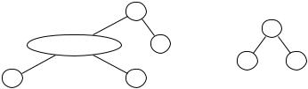
Example 1.23. Consider the formula

F : (P → Q) P ¬Q .

To compute sat F , choose a variable, say P , and recurse on the first case,

F {P 7→ }: ( → Q) ¬Q ,

which simplifies to

Fig. 1.1. Visualizing runs of sat

F1 : Q ¬Q .

Now try each of

F1{Q 7→ } and F1{Q 7→ }.

Both simplify to , so this branch ends without finding a satisfying interpretation.

Now try the other branch for P in F :

F {P 7→ }: ( → Q) ¬Q ,

which simplifies to . Thus, this branch also ends without finding a satisfying interpretation. Thus, F is unsatisfiable.

The run of sat on F is visualized in Figure 1.1(a).

Example 1.24. Consider the formula

F : (P → Q) ¬P .

To compute sat F , choose a variable, say P , and recurse on the first case,

F {P 7→ }: ( → Q) ¬ ,

which simplifies to . Therefore, try

F {P 7→ }: ( → Q) ¬

instead, which simplifies to . Arbitrarily assigning a value to Q produces the following satisfying interpretation:

I : {P 7→false, Q 7→true} .

R

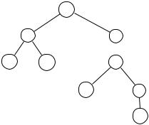
Fig. 1.2. Parse tree of F : P Q → ¬(P ¬R) with representatives for subformulae

1.7.3 Conversion to an Equisatisfiable Formula in CNF

The next two decision procedures operate on PL formulae in CNF. The transformation suggested in Section 1.6 produces an equivalent formula that can be exponentially larger than the original formula: consider converting a formula in DNF into CNF. However, to decide the satisfiability of F , we need only examine a formula F ′ such that F and F ′ are equisatisfiable. F and F ′ are equisatisfiable when F is satisfiable i F ′ is satisfiable.

We define a method for converting PL formula F to equisatisfiable PL formula F ′ in CNF that is at most a constant factor larger than F . The main idea is to introduce new propositional variables to represent the subformulae of F . The constructed formula F ′ includes extra clauses that assert that these new variables are equivalent to the subformulae that they represent.

Figure 1.2 visualizes the idea of the procedure. Each node of the “parse tree” of F represents a subformula G of F . With each node G is associated a representative propositional variable Rep(G). In the constructed formula F ′, each representative Rep(G) is asserted to be equivalent to the subformula G that it represents in such a way that the conjunction of all such assertions is in CNF. Finally, the representative Rep(F ) of F is asserted to be true.

To obtain a small formula in CNF, each assertion of equivalence between Rep(G) and G refers at most to the children of G in the parse tree. How is this possible when a subformula may be arbitrarily large? The main trick is to refer to the representatives of G’s children rather than the children themselves.

Let the “representative” function Rep : PL → V { , } map PL formulae to propositional variables V, , or . In the general case, it is intended to map a formula F to its representative propositional variable PF such that the truth value of PF is the same as that of F . In other words, PF provides a compact way of referring to F .

Let the “encoding” function En : PL → PL map PL formulae to PL formulae. En is intended to map a PL formula F to a PL formula F ′ in CNF that asserts that F ’s representative, PF , is equivalent to F : “Rep(F ) ↔ F ”.

As the base cases for defining Rep and En, define their behavior on , , and propositional variables P :

The representative of is itself, and the representative of is itself. Thus, Rep( ) ↔ and Rep( ) ↔ are both trivially valid, so En( ) and En( ) are both . Finally, the representative of a propositional variable P is P itself; and again, Rep(P ) ↔ P is trivially valid so that En(P ) is .

For the inductive case, F is a formula other than an atom, so define its representative as a unique propositional variable PF :

Rep(F ) = PF .

En then asserts the equivalence of F and PF as a CNF formula. On conjunction, define

En(F1 F2) =

let P = Rep(F1 F2) in

(¬P Rep(F1)) (¬P Rep(F2)) (¬Rep(F1) ¬Rep(F2) P ) The returned formula

(¬P Rep(F1)) (¬P Rep(F2)) (¬Rep(F1) ¬Rep(F2) P )

is in CNF and is equivalent to

Rep(F1 F2) ↔ Rep(F1) Rep(F2) .

In detail, the first two clauses

(¬P Rep(F1)) (¬P Rep(F2))

together assert

P → Rep(F1) Rep(F2)

(since, for example, ¬P Rep(F1) is equivalent to P → Rep(F1)), while the final clause asserts

Rep(F1) Rep(F2) → P .

Notice the application of Rep to F1 and F2. As mentioned above, it is the trick to producing a small CNF formula.

On negation, En(¬F ) returns a formula equivalent to Rep(¬F ) ↔ ¬Rep(F ):

En(¬F ) =

let P = Rep(¬F ) in

(¬P ¬Rep(F )) (P Rep(F ))

Having defined En, let us construct the full CNF formula that is equisatisfiable to F . If SF is the set of all subformulae of F (including F itself), then

is in CNF and is equisatisfiable to F . The second main conjunct asserts the equivalences between all subformulae of F and their corresponding representatives. Rep(F ) asserts that F ’s representative, and thus F itself (according to the second conjunct), is true.

If F has size n, where each instance of a logical connective or a propositional variable contributes one unit of size, then F ′ has size at most 30n + 2. The size of F ′ is thus linear in the size of F . The number of symbols in the formula returned by En(F1 ↔ F2), which incurs the largest expansion, is 29. Up to one additional conjunction is also required per symbol of F . Finally, two extra symbols are required for asserting that Rep(F ) is true.

Example 1.25. Consider formula

F : (Q1 Q2) (R1 R2) ,

which is in DNF. To convert it to CNF, we collect its subformulae

SF : {Q1, Q2, Q1 Q2, R1, R2, R1 R2, F }

and compute

En(Q1) =

En(Q2) =

En(Q1 Q2) = (¬P(Q1 Q2) Q1) (¬P(Q1 Q2 ) Q2)

(¬Q1 ¬Q2 P(Q1 Q2 ))

En(R1) =

En(R2) =

En(R1 R2) = (¬P(R1 R2) R1) (¬P(R1 R2) R2)

(¬R1 ¬R2 P(R1 R2))

En(F ) = (¬P(F ) P(Q1 Q2) P(R1 R2))

(¬P(Q1 Q2) P(F ))

(¬P(R1 R2) P(F ))

1.7.4 The Resolution Procedure

The next decision procedure that we consider is based on resolution and applies only to PL formulae in CNF. Therefore, the procedure of Section 1.7.3 must first be applied to the given PL formula if it is not already in CNF.

Resolution follows from the following observation of any PL formula F in CNF: to satisfy clauses C1[P ] and C2[¬P ] that share variable P but disagree on its value, either the rest of C1 or the rest of C2 must be satisfied. Why? If P is true, then a literal other than ¬P in C2 must be satisfied; while if P is false, then a literal other than P in C1 must be satisfied. Therefore, the clause C1[ ] C2[ ], simplified according to the template equivalences of Exercise 1.2, can be added as a conjunction to F to produce an equivalent formula still in CNF.

Clausal resolution is stated as the following proof rule:

C1[P ] C2[¬P ]

C1[ ] C2[ ]

From the two clauses of the premise, deduce the new clause, called the resolvent.

If ever is deduced via resolution, F must be unsatisfiable since F is unsatisfiable. Otherwise, if every possible resolution produces a clause that is already known, then F must be satisfiable.

Example 1.26. The CNF of (P → Q) P ¬Q is the following:

F : (¬P Q) P ¬Q .