3. Операции

3.1. Поиск

Операция поиска в scapegoat-деревьях осуществляется как в обычных деревьях двоичного поиска. Перестройка дерева не выполняется.

3.2. Вставка

Вставляя узел в дерево со штрафами, мы вставляем его как в обычное бинарное дерево, увеличиваем size[T] и устанавливаем max_size[T] как максимум между size[T] и max_size[T]. Далее если нововставленный узел глубокий – мы балансируем дерево следующим образом. Пусть x0 – нововсталенный глубокий узел и обозначим  x_i+1 как предка x_i.  Мы поднимаемся по дереву, рассматривая x₀, x₁, x₂, и так далее, пока не найдем узел x_i, который не α-weight-сбалансированным. Поскольку x₀ является листом, то size(x_i)=0. Мы вычисляем size(x_j+1), используя формулу

size(x_j+1) = size(x_j) + size(brother(x_j)) + 1 при j=1,2..i

Мы называем x_i предком x₀, которое было найдено как не α -weight-сбалансированно, узел scapegoat (козел отпущения). Этот узел должен существовать по лемме (*), приведенной  ниже.

Когда scapegoat узел x_i найден, мы перестраиваем поддерево с корнем в x_i. Перестройка поддерева это перемещение его ½-weight-сбалансированным поддеревом, содержащим те же узлы. Это легко осуществляется за время O(size(x_i)). Вообще говоря, эта операция может быть осуществлена за время O(log n).

3.3. Удаление

Деревья со штрафами необычны тем, что удаление легче, чем вставка. Удаление осуществляется также как удаление в простых бинарных деревьях поиска  – узел просто помечается как удаленный и по нему не происходит поиск, но вместе с этим мы уменьшаем size[T]. Когда size[T] < α * max_size[T] мы перестраиваем все дерево и сбрасываем max_size[T] в size[T]. Удаление происходит в худшем случае за время О(n), однако это амортизируются как O (log n).  Фактически удаленные узлы изымаются из дерева со штрафами в момент перестройки дерева.

В большинстве случаев могут быть выполнено n/2  – 1 операций удаления, прежде чем дерево должно быть перестроено. Стоимость каждого из этих удалений равна O(log n) (количество времени для поиска элемента и пометка, что он удален). При количестве операции удаления n/2 следует перестроить дерево. Это занимает О(log n) + O (n) (или просто O (n)) времени. Использование совокупного анализа становится ясно, что амортизированная стоимость удаления равна O (log n).

3.4. Замечания

• Каждый раз, когда происходит полная перестройка дерева max_size[T] устанавливается равным size[T].

• Заметим, что ha(T) легко вычисляется по информации, хранящейся в корне дерева.

• Нам не нужны явные поля предков в узлах дерева со штрафами, так как мы поднимаемся обратно вверх по тропинке, по которой спустились, чтобы вставить новый узел; узлы xi в этом пути можно запомнить в стек.

Лемма (*)

Если x это узел на глубине, большей чем h_α (T), то это α -weight-несбалансированный предок x

In computer science, a scapegoat tree is a self-balancing binary search tree, discovered by Arne Anderson^[1] and again by Igal Galperin and Ronald L. Rivest.^[2] It provides worst-case O(log n) lookup time, and O(log n) amortized insertion and deletion time.

Unlike most other self-balancing binary search trees that provide worst case O(log n) lookup time, scapegoat trees have no additional per-node memory overhead compared to a regular binary search tree: a node stores only a key and two pointers to the child nodes. This makes scapegoat trees easier to implement and, due to data structure alignment, can reduce node overhead by up to one-third.

Contents   [hide]  1 Theory 2 Operations 2.1 Insertion 2.2 Sketch of proof for cost of insertion 2.3 Deletion 2.3.1 Sketch of proof for cost of deletion 2.4 Lookup 3 See also 4 References 5 External links

[edit]Theory

A binary search tree is said to be weight balanced if half the nodes are on the left of the root, and half on the right. An α-weight-balanced is therefore defined as meeting the following conditions:

size(left) <= α*size(node)

size(right) <= α*size(node)

Where size can be defined recursively as:

function size(node)

if node = nil

return 0

else

return size(node->left) + size(node->right) + 1

end

An α of 1 therefore would describe a linked list as balanced, whereas an α of 0.5 would only match almost complete binary trees.

A binary search tree that is α-weight-balanced must also be α-height-balanced, that is

height(tree) <= log_1/α(NodeCount)

Scapegoat trees are not guaranteed to keep α-weight-balance at all times, but are always loosely α-height-balance in that

height(scapegoat tree) <= log_1/α(NodeCount) + 1

This makes scapegoat trees similar to red-black trees in that they both have restrictions on their height. They differ greatly though in their implementations of determining where the rotations (or in the case of scapegoat trees, rebalances) take place. Whereas red-black trees store additional 'color' information in each node to determine the location, scapegoat trees find a scapegoat which isn't α-weight-balanced to perform the rebalance operation on. This is loosely similar to AVL trees, in that the actual rotations depend on 'balances' of nodes, but the means of determining the balance differs greatly. Since AVL trees check the balance value on every insertion/deletion, it is typically stored in each node; scapegoat trees are able to calculate it only as needed, which is only when a scapegoat needs to be found.

Unlike most other self-balancing search trees, scapegoat trees are entirely flexible as to their balancing. They support any α such that 0.5 < α < 1. A high α value results in fewer balances, making insertion quicker but lookups and deletions slower, and vice versa for a low α. Therefore in practical applications, an α can be chosen depending on how frequently these actions should be performed.

[edit]Operations

[edit]Insertion

Insertion is implemented with the same basic ideas as an unbalanced binary search tree, however with a few significant changes.

When finding the insertion point, the depth of the new node must also be recorded. This is implemented via a simple counter that gets incremented during each iteration of the lookup, effectively counting the number of edges between the root and the inserted node. If this node violates the α-height-balance property (defined above), a rebalance is required.

To rebalance, an entire subtree rooted at a scapegoat undergoes a balancing operation. The scapegoat is defined as being an ancestor of the inserted node which isn't α-weight-balanced. There will always be at least one such ancestor. Rebalancing any of them will restore the α-height-balanced property.

One way of finding a scapegoat, is to climb from the new node back up to the root and select the first node that isn't α-weight-balanced.

Climbing back up to the root requires O(log n) storage space, usually allocated on the stack, or parent pointers. This can actually be avoided by pointing each child at its parent as you go down, and repairing on the walk back up.

To determine whether a potential node is a viable scapegoat, we need to check its α-weight-balanced property. To do this we can go back to the definition:

size(left) <= α*size(node)

size(right) <= α*size(node)

However a large optimisation can be made by realising that we already know two of the three sizes, leaving only the third having to be calculated.

Consider the following example to demonstrate this. Assuming that we're climbing back up to the root:

size(parent) = size(node) + size(sibling) + 1

But as:

size(inserted node) = 1.

The case is trivialized down to:

size[x+1] = size[x] + size(sibling) + 1

Where x = this node, x + 1 = parent and size(sibling) is the only function call actually required.

Once the scapegoat is found, the subtree rooted at the scapegoat is completely rebuilt to be perfectly balanced.^[2] This can be done in O(n) time by traversing the nodes of the subtree to find their values in sorted order and recursively choosing the median as the root of the subtree.

As rebalance operations take O(n) time (dependent on the number of nodes of the subtree), insertion has a worst case performance of O(n) time. However, because these worst-case scenarios are spread out, insertion takes O(log n) amortized time.

[edit]Sketch of proof for cost of insertion

Define the Imbalance of a node v to be the absolute value of the difference in size between its left node and right node minus 1, or 0, whichever is greater. In other words:

Immediately after rebuilding a subtree rooted at v, I(v) = 0.

Lemma: Immediately before rebuilding the subtree rooted at v, ( is Big O Notation.)

Proof of lemma:

Let be the root of a subtree immediately after rebuilding. . If there are degenerate insertions (that is, where each inserted node increases the height by 1), then , and .

Since before rebuilding, there were insertions into the subtree rooted at that did not result in rebuilding. Each of these insertions can be performed in time. The final insertion that causes rebuilding costs . Using aggregate analysis it becomes clear that the amortized cost of an insertion is :

[edit]Deletion

Scapegoat trees are unusual in that deletion is easier than insertion. To enable deletion, scapegoat trees need to store an additional value with the tree data structure. This property, which we will call MaxNodeCount simply represents the highest achieved NodeCount. It is set to NodeCount whenever the entire tree is rebalanced, and after insertion is set to max(MaxNodeCount, NodeCount).

To perform a deletion, we simply remove the node as you would in a simple binary search tree, but if

NodeCount <= MaxNodeCount / 2

then we rebalance the entire tree about the root, remembering to set MaxNodeCount to NodeCount.

This gives deletion its worst case performance of O(n) time, however it is amortized to O(log n) average time.

[edit]Sketch of proof for cost of deletion

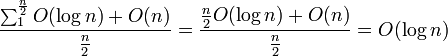
Suppose the scapegoat tree has elements and has just been rebuilt (in other words, it is a complete binary tree). At most deletions can be performed before the tree must be rebuilt. Each of these deletions take time (the amount of time to search for the element and flag it as deleted). The deletion causes the tree to be rebuilt and takes (or just ) time. Using aggregate analysis it becomes clear that the amortized cost of a deletion is :

[edit]Lookup

Lookup is not modified from a standard binary search tree, and has a worst-case time of O(log n). This is in contrast to splay trees which have a worst-case time of O(n). The reduced node memory overhead compared to other self-balancing binary search trees can further improve locality of reference and caching.

В компьютерной науке , козлом отпущения дерево является самостоятельным балансом двоичного дерева поиска , обнаруженных Арне Андерсона ^[ 1 ] и снова Игаль Гальперин и Рональд Л. Rivest . ^[ 2 ] Она предоставляет худшем случае O (журнал N ) время поиска, и O(журнал N ) амортизированной вставки и удаления времени.

В отличие от большинства других самостоятельном балансе двоичные деревья поиска, которые обеспечивают худшем случае O (журнал N ) время поиска, козлом отпущения деревья не имеют дополнительных каждого узла памяти, накладные расходы по сравнению с обычным бинарное дерево поиска : узел хранит только ключом и два указателя на дочерних узлов. Это делает козлом отпущения деревья проще в реализации и, в связи с выравниванием структуры данных , может снизить накладные расходы узла до одной трети.

Содержание   [ скрыть ]  1 Теория 2 операции 2,1 Insertion 2,2 Набросок доказательства по стоимости вставка 2,3 удалений 2.3.1 Схема доказательства стоимости удаления 2,4 Lookup 3 См. также 4 Список литературы 5 Внешние ссылки