МИНИСТЕРСТВО ОБЩЕГО И ПРОФЕССИОНАЛЬНОГО ОБРАЗОВАНИЯ РОССИЙСКОЙ ФЕДЕРАЦИИ
Государственный Университет Управления
Кафедра Экономической кибернетики
Лабораторная работа №1 по дисциплине:
«Методы социально-экономического прогнозирования»
На тему:
«Анализ одномерных временных рядов»
Выполнил: студент ИИСУ
специальности ММиИОЭ IV-1
Мирончук Евгений
Проверила: Писарева О.М.
Москва 1999
Исходные данные для выполнения лабораторной работы №1 представлены в Приложении №1
Последовательность выполнения каждого этапа задания: на основе исходных данных временного ряда (30 значений) необходимо построить прогноз на один период вперед (на 31 период). Чтобы построить более точный прогноз предполагается провести ряд опытов. Для этого исходный ряд разбивается на два участка: тестовый (25 значений) и проверочный (5 последних значений исх. ряда). Используя методы прогнозирования, на основе значений тестового участка строим прогноз на 5 периодов вперед. Затем, сравнивая прогнозные значения со значениями проверочного участка исходного ряда, выбираем наилучший метод и модель прогнозирования, с помощью которых и будет построен прогноз на 31 период.
Этап 1. Сглаживание временного ряда методом простой скользящей средней. Оценка точности прогнозирования уровня показателя.
Для определение расчетных значений показателя используется следующая формула:

где m – продолжительность интервала сглаживания.
В данной работе сглаживание производится для m=3,5,7,9,11,13
Для построения прогнозов используется
адаптивная скользящая средняя
![]()
Результаты сглаживания и построения прогнозов смотрите в Приложениях № 2-3.
Для оценки точности прогноза используется коэффициент несоответствия:
![]() ,
где L - продолжительность периода
упреждения
,
где L - продолжительность периода
упреждения
Чем ближе КТ к нулю, тем совершеннее прогноз. Коэффициенты несоответствия для построенных прогнозов приведены в таблице:
|
p |
Simple Moving Average |
|
KT |
|
|
1 (m=3) |
0,223 |
|
2 (m=5) |
0,232 |
|
3 (m=7) |
0,286 |
|
4 (m=9) |
0,430 |
|
5 (m=11) |
0,529 |
|
6 (m=13) |
0,629 |
Видно, что наименьшее значение KT получается при продолжительности интервала сглаживая m=3 (p=1). Следовательно, прогноз на 31 период будем строить при m = 3 (по исходному ряду).
Точечный прогноз (см. Приложение №
4): ![]()
Интервальная оценка прогноза:
![]()
![]()
![]()
Этап 2. Сглаживание временного ряда с использованием модели Брауна (экспоненциальное сглаживание). Оценка точности прогнозирования уровня показателя.
Для определение расчетных значений показателя используется следующая формула:
![]() ,
где - параметр
определяющий влияние устаревших данных
на сглаживаемый показатель.
,
где - параметр
определяющий влияние устаревших данных
на сглаживаемый показатель.
Прогнозирование с помощью процедур экспоненциального сглаживания осуществляется с помощью так называемых прогнозирующих полиномов. Прогноз уровня ряда yt на период t+ может быть представлен в виде:
![]() , где
- период упреждения
, где
- период упреждения
N – степень аппроксимирующего полинома
При N=0 ![]() (Simple
Exp. Smoothing)
(Simple
Exp. Smoothing)
При N=1 ![]() (Linear
Exp. Smoothing)
(Linear
Exp. Smoothing)
При N=2 ![]() (Quadratic
Exp. Smoothing)
(Quadratic
Exp. Smoothing)
Результаты построения 5-ти прогнозных значений с использованием Simple Exp. Smoothing приведены в Приложении № 5. Результаты оценки точности прогнозных значений со значениями проверочного участка представлены в таблице:
|
|
Simple Exp. Smoothing |
|
|
S |
KT |
|
|
0,1 |
18,72 |
0,507 |
|
0,2 |
15,32 |
0,373 |
|
0,3 |
12,96 |
0,256 |
|
0,4 |
11,35 |
0,216 |
|
0,5 |
10,28 |
0,213 |
|
0,6 |
9,57 |
0,220 |
|
0,7 |
9,09 |
0,229 |
|
0,8 |
8,76 |
0,233 |
|
0,9 |
8,53 |
0,238 |
Из таблицы видно, что наилучший прогноз получается при = 0,5. Прогноз на 31 период строим при = 0,5 (см. Приложение № 6).
Точечный прогноз: ![]()
Интервальная оценка прогноза:
![]()
![]()
Результаты построения прогнозных значений на 5 периодов вперед с использованием Linear Exp. Smoothing приведены в Приложении № 7. Результаты оценки точности прогноза представлены в таблице:
|
|
Linear Exp. Smoothing |
|
|
S |
KT |
|
|
0,1 |
16,23 |
0,508 |
|
0,2 |
12,93 |
0,338 |
|
0,3 |
10,28 |
0,647 |
|
0,4 |
9,21 |
0,754 |
|
0,5 |
8,99 |
0,720 |
|
0,6 |
9,13 |
0,632 |
|
0,7 |
9,42 |
0,545 |
|
0,8 |
9,83 |
0,484 |
|
0,9 |
10,37 |
0,449 |
КТ принимает минимальное значение при = 0,2.
Результаты построения прогнозного значение на 31 период приведены в Приложении № 8:
Точечный прогноз: ![]()
Интервальная оценка
прогноза: ![]()
Результаты построения прогнозных значений на 5 периодов вперед с использованием Quadratic Exp. Smoothing смотрите в Приложении № 9. Результаты оценки точности прогноза представлены в таблице:
|
|
Quadratic Exp. Smoothing |
|
|
S |
KT |
|
|
0,1 |
16,03 |
0,305 |
|
0,2 |
11,46 |
1,083 |
|
0,3 |
9,54 |
1,236 |
|
0,4 |
9,69 |
0,831 |
|
0,5 |
10,39 |
0,328 |
|
0,6 |
11,31 |
0,139 |
|
0,7 |
12,43 |
0,219 |
|
0,8 |
13,87 |
0,144 |
|
0,9 |
15,87 |
0,152 |
В данном случае минимальному значению КТ соответствует =0,6
Результаты прогнозирования на 31 период приведены в Приложении № 10:
Точечный прогноз: ![]()
Интервальная оценка
прогноза: ![]()
Этап 3. Сглаживание временного ряда с использованием модели тренда. Оценка точности прогнозирования уровня показателя.
Уровни временного ряда в данном случае могут быть описаны следующим уравнением:
![]()
Прогнозные значения показателя yt рассчитываются по формуле:
![]() ,
где l=1,L
,
где l=1,L
Для прогнозирования на основе модели линейного тренда доверительный интервал определяется по формуле:
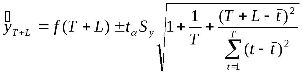
или
![]()
![]()
Однако, перед тем как использовать модели трендов необходимо проверить гипотезы о существовании тенденции в развитии.
Сформулируем основную гипотезу (гипотеза о наличии тенденции в средних):
![]()
 tтабл
(0,05;n+m-2)
tтабл
(0,05;n+m-2)
Если t>tкр принимаем гипотезу H1, тенденция в средних есть.
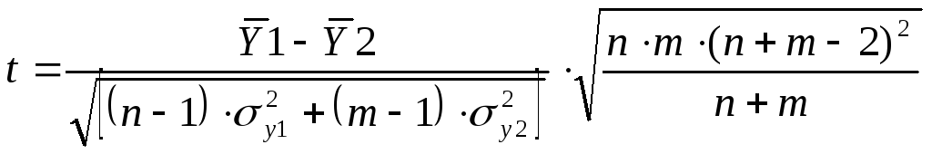
Перед проверкой основной гипотезы необходимо сформулировать и проверить вспомогательную (гипотеза о проверки однородности ряда):
![]()
![]()
![]()
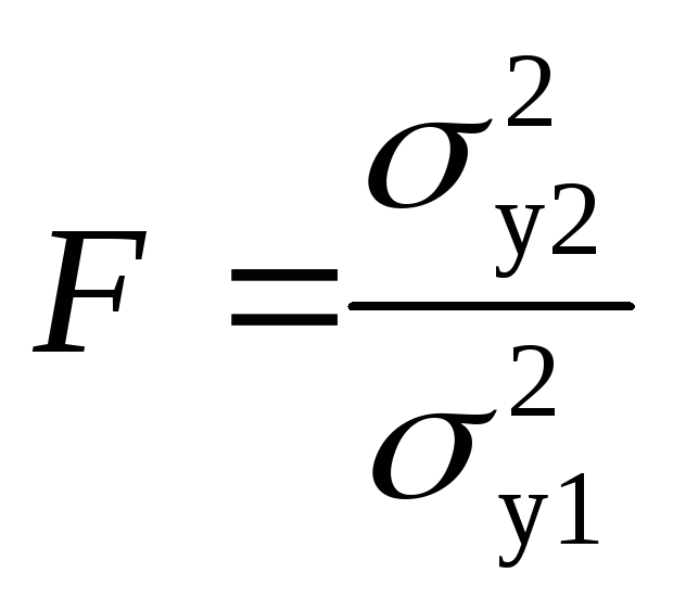 Fтабл
(0.05;m-1;n-1)
Fтабл
(0.05;m-1;n-1)
Если F<Fтабл принимаем гипотезу H0, совокупность однородная
В данной работе было выполнено 16 различных разбиений тестового ряда (первые 25 значений) на 2 совокупности и проверены вспомогательная и основная гипотезы (см. Приложения № 11-18).
Только в одном случае была выявлена тенденция в средних (основная гипотеза Н1) при одновременной однородности совокупности (вспомогательная гипотеза Н0) (см. Приложение № 13).
Fрасч =1,903404 < Fтабл(0,05;17;6)=3,91 совокупность однородна
tрасч=2,309429 > tтабл(0,05;23)=2,0686 существует тенденция в средних
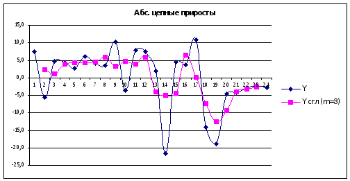
После проверки гипотез можно приступать к построению трендовых моделей. Однако для того, чтобы выбрать модель тренда необходимо определить тип экономического роста. Для этого рассчитаем абсолютные цепные приросты по следующей формуле:
![]()
Результаты расчетов и их графическое изображение представлены в Приложении № 29.
Заметим, что идентификация типа экономического роста, исходя из полученных результатов, представляется достаточно непростой задачей. Поэтому просто построим ряд простейших трендов и посмотрим их характеристики (см. Приложения № 19-26).
Основные характеристики использованных трендовых моделей, а также оценка качества прогнозов приведены в таблице:
|
№ |
Модели тренда |
Характеристики модели |
|||
|
S2 |
R2 |
Fрасч (Fтабл) |
KT |
||
|
1 |
Y=49,9+0,155*t |
301,186 |
0,00452 |
0,1 (4,297) |
0,682 |
|
2 |
Y=exp(3,87+0,002*t) |
0,118 |
0,00182 |
0,04 (4,297) |
0,582 |
|
3 |
Y=exp(4,0-0,696/t) |
0,0968 |
0,182 |
5,12 (4,297) |
0,659 |
|
4 |
Y=12,34+8,5*t-0,32*t^2 |
62,6173 |
0,802 |
44,57 (3,44) |
1,199 |
|
5 |
Y=1/(0,02+0,015/t) |
0,000043 |
0,198 |
5,69 (4,297) |
0,589 |
|
6 |
Y=39,6-7,3t+2,0t^2-0,13t^3+0,002t^4 |
39,098 |
0,888 |
39,5 (2,87) |
0,184 |
Из таблицы видно, что лучшими прогнозными (по KT ) и модельными (по R2 ) характеристиками обладает полином 4 порядка (модель № 6).
Линейная (№1) и экспоненциальная (№2) модели вообще говоря незначимы, так как Fрасч<Fтабл. Это подтверждает тот факт, что использовать эти модели в данном случае не следовало бы.
Итак, для построения прогноза на 31 период по исходному временному ряду используем полином 4-го порядка. Результаты построения смотрите в Приложении № 27 :
Точечный прогноз: ![]()
Интервальная оценка
прогноза: ![]()
Все варианты прогнозных значений, полученных в этой лабораторной работе, можно наглядно увидеть на диаграмме, представленной в Приложении № 28. Как видно, полученные значения существенно отличаются друг от друга, и не дают возможности однозначно определить поведения исследуемой системы в будущем. Вероятнее всего в данном случае нужно применять другие методы и модели для построения прогноза.
Приложения
Приложение №1
|
|
|
t |
Y |
|
Ретроспективный период |
Тестовый участок |
1 |
30,0 |
|
2 |
37,4 |
||
|
3 |
31,9 |
||
|
4 |
36,7 |
||
|
5 |
41,0 |
||
|
6 |
43,7 |
||
|
7 |
49,7 |
||
|
8 |
53,9 |
||
|
9 |
57,4 |
||
|
10 |
67,6 |
||
|
11 |
63,9 |
||
|
12 |
71,8 |
||
|
13 |
79,3 |
||
|
14 |
81,3 |
||
|
15 |
59,6 |
||
|
16 |
64,2 |
||
|
17 |
67,9 |
||
|
18 |
78,8 |
||
|
19 |
64,6 |
||
|
20 |
45,7 |
||
|
21 |
41,0 |
||
|
22 |
36,8 |
||
|
23 |
33,9 |
||
|
24 |
31,6 |
||
|
25 |
28,7 |
||
|
Проверочный участок |
26 |
26,7 |
|
|
27 |
25,1 |
||
|
28 |
29 |
||
|
29 |
39,7 |
||
|
30 |
42,4 |

Приложение №2
(Simple Moving Average)
|
t |
Y |
|
Y^ |
m=3 (p=1) |
Y^ |
m=5 (p=2) |
Y^ |
m=7 (p=3) |
||||||||||||
|
1 |
30,0 |
|
30,0 |
|
|
|
|
|
30,0 |
|
|
|
|
|
30,0 |
|
|
|
|
|
|
2 |
37,4 |
|
37,4 |
|
|
|
|
|
37,4 |
|
|
|
|
|
37,4 |
|
|
|
|
|
|
3 |
31,9 |
|
31,9 |
|
|
|
|
|
31,9 |
|
|
|
|
|
31,9 |
|
|
|
|
|
|
4 |
36,7 |
|
36,7 |
|
|
|
|
|
36,7 |
|
|
|
|
|
36,7 |
|
|
|
|
|
|
5 |
41,0 |
|
41,0 |
|
|
|
|
|
41,0 |
|
|
|
|
|
41,0 |
|
|
|
|
|
|
6 |
43,7 |
|
43,7 |
|
|
|
|
|
43,7 |
|
|
|
|
|
43,7 |
|
|
|
|
|
|
7 |
49,7 |
|
49,7 |
|
|
|
|
|
49,7 |
|
|
|
|
|
49,7 |
|
|
|
|
|
|
8 |
53,9 |
|
53,9 |
|
|
|
|
|
53,9 |
|
|
|
|
|
53,9 |
|
|
|
|
|
|
9 |
57,4 |
|
57,4 |
|
|
|
|
|
57,4 |
|
|
|
|
|
57,4 |
|
|
|
|
|
|
10 |
67,6 |
|
67,6 |
|
|
|
|
|
67,6 |
|
|
|
|
|
67,6 |
|
|
|
|
|
|
11 |
63,9 |
|
63,9 |
|
|
|
|
|
63,9 |
|
|
|
|
|
63,9 |
|
|
|
|
|
|
12 |
71,8 |
|
71,8 |
|
|
|
|
|
71,8 |
|
|
|
|
|
71,8 |
|
|
|
|
|
|
13 |
79,3 |
|
79,3 |
|
|
|
|
|
79,3 |
|
|
|
|
|
79,3 |
|
|
|
|
|
|
14 |
81,3 |
|
81,3 |
|
|
|
|
|
81,3 |
|
|
|
|
|
81,3 |
|
|
|
|
|
|
15 |
59,6 |
|
59,6 |
|
|
|
|
|
59,6 |
|
|
|
|
|
59,6 |
|
|
|
|
|
|
16 |
64,2 |
|
64,2 |
|
|
|
|
|
64,2 |
|
|
|
|
|
64,2 |
|
|
|
|
|
|
17 |
67,9 |
|
67,9 |
|
|
|
|
|
67,9 |
|
|
|
|
|
67,9 |
|
|
|
|
|
|
18 |
78,8 |
|
78,8 |
|
|
|
|
|
78,8 |
|
|
|
|
|
78,8 |
|
|
|
|
|
|
19 |
64,6 |
|
64,6 |
|
|
|
|
|
64,6 |
|
|
|
|
|
64,6 |
|
|
|
|
|
|
20 |
45,7 |
|
45,7 |
|
|
|
|
|
45,7 |
|
|
|
|
|
45,7 |
|
|
|
|
|
|
21 |
41,0 |
|
41,0 |
|
|
|
|
|
41,0 |
|
|
|
|
|
41,0 |
|
|
|
|
|
|
22 |
36,8 |
|
36,8 |
|
|
|
|
|
36,8 |
|
|
|
|
|
36,8 |
40,3 |
|
|
|
|
|
23 |
33,9 |
|
33,9 |
|
|
|
|
|
33,9 |
34,4 |
|
|
|
|
33,9 |
|
36,9 |
|
|
|
|
24 |
31,6 |
|
31,6 |
31,4 |
|
|
|
|
31,6 |
|
33,1 |
|
|
|
31,6 |
|
|
35,6 |
|
|
|
25 |
28,7 |
|
28,7 |
|
30,6 |
|
|
|
28,7 |
|
|
32,3 |
|
|
28,7 |
|
|
|
34,8 |
|
|
26 |
26,7 |
|
31,4 |
|
|
30,2 |
|
|
34,4 |
|
|
|
32,0 |
|
40,3 |
|
|
|
|
34,5 |
|
27 |
25,1 |
|
30,6 |
|
|
|
30,7 |
|
33,1 |
|
|
|
|
32,1 |
36,9 |
|
|
|
|
|
|
28 |
29 |
|
30,2 |
|
|
|
|
30,5 |
32,3 |
|
|
|
|
|
35,6 |
|
|
|
|
|
|
29 |
39,7 |
|
30,7 |
|
|
|
|
|
32,0 |
|
|
|
|
|
34,8 |
|
|
|
|
|
|
30 |
42,4 |
|
30,5 |
|
|
|
|
|
32,1 |
|
|
|
|
|
34,5 |
|
|
|
|
|
|
|
|
Кт = |
0,223 |
|
|
|
|
|
0,232 |
|
|
|
|
|
0,286 |
|
|
|
|
|
Приложение №3
(Simple Moving Average)
|
|
Y^ |
m=9 (p=4) |
Y^ |
m=11 (p=5) |
Y^ |
m=13 (p=6) |
||||||||||||
|
|
30,0 |
|
|
|
|
|
30,0 |
|
|
|
|
|
30,0 |
|
|
|
|
|
|
|
37,4 |
|
|
|
|
|
37,4 |
|
|
|
|
|
37,4 |
|
|
|
|
|
|
|
31,9 |
|
|
|
|
|
31,9 |
|
|
|
|
|
31,9 |
|
|
|
|
|
|
|
36,7 |
|
|
|
|
|
36,7 |
|
|
|
|
|
36,7 |
|
|
|
|
|
|
|
41,0 |
|
|
|
|
|
41,0 |
|
|
|
|
|
41,0 |
|
|
|
|
|
|
|
43,7 |
|
|
|
|
|
43,7 |
|
|
|
|
|
43,7 |
|
|
|
|
|
|
|
49,7 |
|
|
|
|
|
49,7 |
|
|
|
|
|
49,7 |
|
|
|
|
|
|
|
53,9 |
|
|
|
|
|
53,9 |
|
|
|
|
|
53,9 |
|
|
|
|
|
|
|
57,4 |
|
|
|
|
|
57,4 |
|
|
|
|
|
57,4 |
|
|
|
|
|
|
|
67,6 |
|
|
|
|
|
67,6 |
|
|
|
|
|
67,6 |
|
|
|
|
|
|
|
63,9 |
|
|
|
|
|
63,9 |
|
|
|
|
|
63,9 |
|
|
|
|
|
|
|
71,8 |
|
|
|
|
|
71,8 |
|
|
|
|
|
71,8 |
|
|
|
|
|
|
|
79,3 |
|
|
|
|
|
79,3 |
|
|
|
|
|
79,3 |
|
|
|
|
|
|
|
81,3 |
|
|
|
|
|
81,3 |
|
|
|
|
|
81,3 |
|
|
|
|
|
|
|
59,6 |
|
|
|
|
|
59,6 |
|
|
|
|
|
59,6 |
|
|
|
|
|
|
|
64,2 |
|
|
|
|
|
64,2 |
|
|
|
|
|
64,2 |
|
|
|
|
|
|
|
67,9 |
|
|
|
|
|
67,9 |
|
|
|
|
|
67,9 |
|
|
|
|
|
|
|
78,8 |
|
|
|
|
|
78,8 |
|
|
|
|
|
78,8 |
|
|
|
|
|
|
|
64,6 |
|
|
|
|
|
64,6 |
|
|
|
|
|
64,6 |
54,9 |
|
|
|
|
|
|
45,7 |
|
|
|
|
|
45,7 |
50,3 |
|
|
|
|
45,7 |
|
53,0 |
|
|
|
|
|
41,0 |
47,7 |
|
|
|
|
41,0 |
|
49,4 |
|
|
|
41,0 |
|
|
50,8 |
|
|
|
|
36,8 |
|
45,4 |
|
|
|
36,8 |
|
|
48,1 |
|
|
36,8 |
|
|
|
50,1 |
|
|
|
33,9 |
|
|
41,7 |
|
|
33,9 |
|
|
|
46,3 |
|
33,9 |
|
|
|
|
49,1 |
|
|
31,6 |
|
|
|
39,2 |
|
31,6 |
|
|
|
|
43,3 |
31,6 |
|
|
|
|
|
|
|
28,7 |
|
|
|
|
38,4 |
28,7 |
|
|
|
|
|
28,7 |
|
|
|
|
|
|
|
47,7 |
|
|
|
|
|
50,3 |
|
|
|
|
|
54,9 |
|
|
|
|
|
|
|
45,4 |
|
|
|
|
|
49,4 |
|
|
|
|
|
53,0 |
|
|
|
|
|
|
|
41,7 |
|
|
|
|
|
48,1 |
|
|
|
|
|
50,8 |
|
|
|
|
|
|
|
39,2 |
|
|
|
|
|
46,3 |
|
|
|
|
|
50,1 |
|
|
|
|
|
|
|
38,4 |
|
|
|
|
|
43,3 |
|
|
|
|
|
49,1 |
|
|
|
|
|
|
Kт = |
0,430 |
|
|
|
|
|
0,529 |
|
|
|
|
|
0,629 |
|
|
|
|
|
Приложение № 4
(Simple Moving Average)
Forecast Table for Y
Model: Simple moving average of 3 terms
Period Data Forecast Residual
------------------------------------------------------------------------------
1,0 30,0
2,0 37,4
3,0 31,9
4,0 36,7 33,1 3,6
5,0 41,0 35,3333 5,66667
6,0 43,7 36,5333 7,16667
7,0 49,7 40,4667 9,23333
8,0 53,9 44,8 9,1
9,0 57,4 49,1 8,3
10,0 67,6 53,6667 13,9333
11,0 63,9 59,6333 4,26667
12,0 71,8 62,9667 8,83333
13,0 79,3 67,7667 11,5333
14,0 81,3 71,6667 9,63333
15,0 59,6 77,4667 -17,8667
16,0 64,2 73,4 -9,2
17,0 67,9 68,3667 -0,466667
18,0 78,8 63,9 14,9
19,0 64,6 70,3 -5,7
20,0 45,7 70,4333 -24,7333
21,0 41,0 63,0333 -22,0333
22,0 36,8 50,4333 -13,6333
23,0 33,9 41,1667 -7,26667
24,0 31,6 37,2333 -5,63333
25,0 28,7 34,1 -5,4
26,0 26,7 31,4 -4,7
27,0 25,1 29,0 -3,9
28,0 29,0 26,8333 2,16667
29,0 39,7 26,9333 12,7667
30,0 42,4 31,2667 11,1333
------------------------------------------------------------------------------
Lower 95,0% Upper 95,0%
Period Forecast Limit Limit
------------------------------------------------------------------------------
31,0 37,0333 12,265 61,8017
------------------------------------------------------------------------------
Forecast Summary
----------------
Forecast model selected: Simple moving average of 3 terms
Number of forecasts generated: 1
Number of periods withheld for validation: 0
Estimation Validation
Statistic Period Period
--------------------------------------------
MSE 119,772
MAE 9,36173
MAPE 19,6547
ME 0,433333
MPE -1,82275
The StatAdvisor
---------------
This model assumes that the best forecast for future data is given by
the average of the 3 most recent data values.You can select a
different forecasting model by pressing the alternate mouse button and
selecting Analysis Options.
The table also summarizes the performance of the currently selected
model in fitting the previous data. It displays:
(1) the mean squared error (MSE)
(2) the mean absolute error (MAE)
(3) the mean absolute percentage error (MAPE)
(4) the mean error (ME)
(5) the mean percentage error (MPE)
Each of the statistics is based on the one-ahead forecast errors,
which are the differences between the data value at time t and the
forecast of that value made at time t-1. The first three statistics
measure the magnitude of the errors. A better model will give a
smaller value. The last two statistics measure bias. A better model
will give a value close to 0.0.
Приложение №5
(Simple Exp. Smoothing)
|
t |
Y |
|
= 0,1 |
= 0,2 |
= 0,3 |
= 0,4 |
= 0,5 |
= 0,6 |
= 0,7 |
= 0,8 |
= 0,9 |
|
1 |
30,0 |
|
30,0 |
30,0 |
30,0 |
30,0 |
30,0 |
30,0 |
30,0 |
30,0 |
30,0 |
|
2 |
37,4 |
|
30,0 |
30,0 |
30,0 |
30,0 |
30,0 |
30,0 |
30,0 |
30,0 |
30,0 |
|
3 |
31,9 |
|
30,7 |
31,5 |
32,2 |
33,0 |
33,7 |
34,4 |
35,2 |
35,9 |
36,7 |
|
4 |
36,7 |
|
30,9 |
31,6 |
32,1 |
32,5 |
32,8 |
32,9 |
32,9 |
32,7 |
32,4 |
|
5 |
41,0 |
|
31,4 |
32,6 |
33,5 |
34,2 |
34,8 |
35,2 |
35,6 |
35,9 |
36,3 |
|
6 |
43,7 |
|
32,4 |
34,3 |
35,7 |
36,9 |
37,9 |
38,7 |
39,4 |
40,0 |
40,5 |
|
7 |
49,7 |
|
33,5 |
36,2 |
38,1 |
39,6 |
40,8 |
41,7 |
42,4 |
43,0 |
43,4 |
|
8 |
53,9 |
|
35,1 |
38,9 |
41,6 |
43,7 |
45,2 |
46,5 |
47,5 |
48,4 |
49,1 |
|
9 |
57,4 |
|
37,0 |
41,9 |
45,3 |
47,8 |
49,6 |
50,9 |
52,0 |
52,8 |
53,4 |
|
10 |
67,6 |
|
39,1 |
45,0 |
48,9 |
51,6 |
53,5 |
54,8 |
55,8 |
56,5 |
57,0 |
|
11 |
63,9 |
|
41,9 |
49,5 |
54,5 |
58,0 |
60,5 |
62,5 |
64,1 |
65,4 |
66,5 |
|
12 |
71,8 |
|
44,1 |
52,4 |
57,3 |
60,4 |
62,2 |
63,3 |
63,9 |
64,2 |
64,2 |
|
13 |
79,3 |
|
46,9 |
56,3 |
61,7 |
64,9 |
67,0 |
68,4 |
69,4 |
70,3 |
71,0 |
|
14 |
81,3 |
|
50,1 |
60,9 |
67,0 |
70,7 |
73,2 |
74,9 |
76,3 |
77,5 |
78,5 |
|
15 |
59,6 |
|
53,2 |
65,0 |
71,3 |
74,9 |
77,2 |
78,8 |
79,8 |
80,5 |
81,0 |
|
16 |
64,2 |
|
53,9 |
63,9 |
67,8 |
68,8 |
68,4 |
67,3 |
65,7 |
63,8 |
61,7 |
|
17 |
67,9 |
|
54,9 |
63,9 |
66,7 |
67,0 |
66,3 |
65,4 |
64,6 |
64,1 |
64,0 |
|
18 |
78,8 |
|
56,2 |
64,7 |
67,1 |
67,3 |
67,1 |
66,9 |
66,9 |
67,1 |
67,5 |
|
19 |
64,6 |
|
58,5 |
67,6 |
70,6 |
71,9 |
73,0 |
74,0 |
75,2 |
76,5 |
77,7 |
|
20 |
45,7 |
|
59,1 |
67,0 |
68,8 |
69,0 |
68,8 |
68,4 |
67,8 |
67,0 |
65,9 |
|
21 |
41,0 |
|
57,7 |
62,7 |
61,9 |
59,7 |
57,2 |
54,8 |
52,3 |
50,0 |
47,7 |
|
22 |
36,8 |
|
56,1 |
58,4 |
55,6 |
52,2 |
49,1 |
46,5 |
44,4 |
42,8 |
41,7 |
|
23 |
33,9 |
|
54,1 |
54,1 |
50,0 |
46,0 |
43,0 |
40,7 |
39,1 |
38,0 |
37,3 |
|
24 |
31,6 |
|
52,1 |
50,0 |
45,1 |
41,2 |
38,4 |
36,6 |
35,5 |
34,7 |
34,2 |
|
25 |
28,7 |
|
50,1 |
46,3 |
41,1 |
37,4 |
35,0 |
33,6 |
32,8 |
32,2 |
31,9 |
|
26 |
26,7 |
|
47,9 |
42,8 |
37,4 |
33,9 |
31,9 |
30,7 |
29,9 |
29,4 |
29,0 |
|
27 |
25,1 |
|
47,9 |
42,8 |
37,4 |
33,9 |
31,9 |
30,7 |
29,9 |
29,4 |
29,0 |
|
28 |
29 |
|
47,9 |
42,8 |
37,4 |
33,9 |
31,9 |
30,7 |
29,9 |
29,4 |
29,0 |
|
29 |
39,7 |
|
47,9 |
42,8 |
37,4 |
33,9 |
31,9 |
30,7 |
29,9 |
29,4 |
29,0 |
|
30 |
42,4 |
|
47,9 |
42,8 |
37,4 |
33,9 |
31,9 |
30,7 |
29,9 |
29,4 |
29,0 |
|
|
|
Кт = |
0,507 |
0,373 |
0,256 |
0,216 |
0,213 |
0,220 |
0,227 |
0,233 |
0,238 |
|
|
|
S^2 = |
350,3 |
234,6 |
167,9 |
128,7 |
105,6 |
91,58 |
82,62 |
76,71 |
72,75 |
|
|
|
|
18,72 |
15,32 |
12,96 |
11,35 |
10,28 |
9,569 |
9,09 |
8,758 |
8,529 |
Приложение №6
(Simple Exp. Smoothing)
Forecast Table for Y
Model: Simple exponential smoothing with alpha = 0,5
Period Data Forecast Residual
------------------------------------------------------------------------------
1,0 30,0 33,4395 -3,43946
2,0 37,4 31,7197 5,68027
3,0 31,9 34,5599 -2,65986
4,0 36,7 33,2299 3,47007
5,0 41,0 34,965 6,03503
6,0 43,7 37,9825 5,71752
7,0 49,7 40,8412 8,85876
8,0 53,9 45,2706 8,62938
9,0 57,4 49,5853 7,81469
10,0 67,6 53,4927 14,1073
11,0 63,9 60,5463 3,35367
12,0 71,8 62,2232 9,57684
13,0 79,3 67,0116 12,2884
14,0 81,3 73,1558 8,14421
15,0 59,6 77,2279 -17,6279
16,0 64,2 68,4139 -4,21395
17,0 67,9 66,307 1,59303
18,0 78,8 67,1035 11,6965
19,0 64,6 72,9517 -8,35174
20,0 45,7 68,7759 -23,0759
21,0 41,0 57,2379 -16,2379
22,0 36,8 49,119 -12,319
23,0 33,9 42,9595 -9,05948
24,0 31,6 38,4297 -6,82974
25,0 28,7 35,0149 -6,31487
26,0 26,7 31,8574 -5,15744
27,0 25,1 29,2787 -4,17872
28,0 29,0 27,1894 1,81064
29,0 39,7 28,0947 11,6053
30,0 42,4 33,8973 8,50266
------------------------------------------------------------------------------
Lower 95,0% Upper 95,0%
Period Forecast Limit Limit
------------------------------------------------------------------------------
31,0 38,1487 19,3014 56,9959
------------------------------------------------------------------------------
Forecast Summary
----------------
Forecast model selected: Simple exponential smoothing with alpha = 0,5
Number of forecasts generated: 1
Number of periods withheld for validation: 0
Estimation Validation
Statistic Period Period
--------------------------------------------
MSE 92,4695
MAE 8,27834
MAPE 17,8778
ME 0,313947
MPE -2,03894
The StatAdvisor
---------------
The table also summarizes the performance of the currently selected
model in fitting the previous data. It displays:
(1) the mean squared error (MSE)
(2) the mean absolute error (MAE)
(3) the mean absolute percentage error (MAPE)
(4) the mean error (ME)
(5) the mean percentage error (MPE)
Приложение №7
(Linear Exp. Smoothing)
|
t |
Y |
|
= 0,1 |
= 0,2 |
= 0,3 |
= 0,4 |
= 0,5 |
= 0,6 |
= 0,7 |
= 0,8 |
= 0,9 |
|
1 |
30,0 |
|
44,8 |
30,8 |
27,4 |
27,6 |
28,1 |
28,2 |
27,6 |
26,5 |
24,9 |
|
2 |
37,4 |
|
41,6 |
28,3 |
26,0 |
26,6 |
27,3 |
27,7 |
28,0 |
28,3 |
28,9 |
|
3 |
31,9 |
|
40,5 |
29,7 |
30,1 |
32,7 |
35,2 |
37,4 |
39,3 |
41,3 |
43,1 |
|
4 |
36,7 |
|
38,4 |
28,8 |
29,5 |
31,3 |
32,2 |
32,3 |
31,7 |
30,5 |
28,7 |
|
5 |
41,0 |
|
37,6 |
30,2 |
32,3 |
34,7 |
36,2 |
37,1 |
37,8 |
38,7 |
39,8 |
|
6 |
43,7 |
|
37,8 |
33,1 |
36,6 |
39,7 |
41,6 |
42,9 |
43,9 |
44,6 |
45,1 |
|
7 |
49,7 |
|
38,5 |
36,3 |
40,7 |
43,9 |
45,5 |
46,4 |
46,8 |
46,9 |
46,7 |
|
8 |
53,9 |
|
40,4 |
41,1 |
46,6 |
50,1 |
52,0 |
53,2 |
53,9 |
54,5 |
55,1 |
|
9 |
57,4 |
|
42,8 |
46,2 |
52,3 |
55,7 |
57,3 |
58,0 |
58,4 |
58,5 |
58,4 |
|
10 |
67,6 |
|
45,6 |
51,1 |
57,4 |
60,2 |
61,2 |
61,5 |
61,5 |
61,3 |
61,1 |
|
11 |
63,9 |
|
50,0 |
58,6 |
65,9 |
69,5 |
71,5 |
72,8 |
74,0 |
75,2 |
76,5 |
|
12 |
71,8 |
|
53,0 |
62,3 |
68,1 |
69,6 |
69,4 |
68,3 |
66,8 |
65,0 |
62,8 |
|
13 |
79,3 |
|
57,1 |
67,9 |
73,5 |
75,1 |
75,4 |
75,5 |
75,8 |
76,5 |
77,8 |
|
14 |
81,3 |
|
62,1 |
74,6 |
80,5 |
82,5 |
83,5 |
84,3 |
85,2 |
86,0 |
86,6 |
|
15 |
59,6 |
|
66,7 |
79,9 |
85,0 |
86,3 |
86,5 |
86,3 |
85,9 |
85,3 |
84,4 |
|
16 |
64,2 |
|
66,3 |
74,7 |
73,9 |
69,5 |
64,2 |
58,8 |
53,3 |
48,0 |
42,8 |
|
17 |
67,9 |
|
66,8 |
72,6 |
69,9 |
65,5 |
62,1 |
60,2 |
59,9 |
61,3 |
64,3 |
|
18 |
78,8 |
|
67,9 |
72,4 |
69,6 |
66,8 |
65,8 |
66,3 |
67,8 |
69,6 |
71,1 |
|
19 |
64,6 |
|
70,9 |
76,4 |
75,9 |
76,2 |
78,1 |
80,9 |
83,8 |
86,3 |
88,2 |
|
20 |
45,7 |
|
70,7 |
73,4 |
70,7 |
68,6 |
67,2 |
65,5 |
62,9 |
59,4 |
55,2 |
|
21 |
41,0 |
|
66,6 |
63,6 |
56,3 |
50,1 |
44,9 |
40,0 |
35,4 |
31,4 |
28,5 |
|
22 |
36,8 |
|
62,2 |
54,7 |
45,4 |
39,0 |
34,8 |
32,3 |
31,4 |
31,9 |
33,7 |
|
23 |
33,9 |
|
57,5 |
46,8 |
37,2 |
32,0 |
29,7 |
29,2 |
29,9 |
31,0 |
32,1 |
|
24 |
31,6 |
|
53,0 |
40,2 |
31,4 |
27,9 |
27,2 |
27,9 |
29,1 |
30,0 |
30,7 |
|
25 |
28,7 |
|
48,6 |
34,7 |
27,4 |
25,5 |
26,0 |
27,1 |
28,1 |
28,8 |
29,1 |
|
26 |
26,7 |
|
48,4 |
32,4 |
23,3 |
20,8 |
21,5 |
23,2 |
24,9 |
26,0 |
26,7 |
|
27 |
25,1 |
|
48,1 |
30,1 |
19,2 |
16,1 |
17,0 |
19,4 |
21,7 |
23,3 |
24,2 |
|
28 |
29 |
|
47,8 |
27,8 |
15,1 |
11,4 |
12,5 |
15,5 |
18,4 |
20,6 |
21,8 |
|
29 |
39,7 |
|
47,5 |
25,4 |
11,0 |
6,6 |
8,0 |
11,6 |
15,2 |
17,8 |
19,3 |
|
30 |
42,4 |
|
47,3 |
23,1 |
6,9 |
1,9 |
3,5 |
7,7 |
12,0 |
15,1 |
16,8 |
|
|
|
Кт = |
0,51 |
0,34 |
0,65 |
0,75 |
0,72 |
0,63 |
0,54 |
0,48 |
0,45 |
|
|
|
S^2 = |
263,4 |
167,3 |
105,7 |
84,8 |
80,9 |
83,4 |
88,8 |
96,6 |
107,4 |
|
|
|
|
16,23 |
12,93 |
10,28 |
9,21 |
8,99 |
9,13 |
9,42 |
9,83 |
10,37 |
Приложение № 8
(Linear Exp. Smoothing)
Forecast Table for Y
Model: Brown's linear exp. smoothing with alpha = 0,2
Period Data Forecast Residual
------------------------------------------------------------------------------
1,0 30,0 30,6777 -0,677734
2,0 37,4 28,1963 9,20369
3,0 31,9 29,6403 2,25965
4,0 36,7 28,6749 8,02508
5,0 41,0 30,106 10,894
6,0 43,7 33,0057 10,6943
7,0 49,7 36,2613 13,4387
8,0 53,9 41,0424 12,8576
9,0 57,4 46,1286 11,2714
10,0 67,6 51,0947 16,5053
11,0 63,9 58,6051 5,29487
12,0 71,8 62,2916 9,50837
13,0 79,3 67,8753 11,4247
14,0 81,3 74,6059 6,69413
15,0 59,6 79,9012 -20,3012
16,0 64,2 74,6661 -10,4661
17,0 67,9 72,5531 -4,65307
18,0 78,8 72,3466 6,45342
19,0 64,6 76,3966 -11,7966
20,0 45,7 73,4047 -27,7047
21,0 41,0 63,5777 -22,5777
22,0 36,8 54,6933 -17,8933
23,0 33,9 46,7796 -12,8796
24,0 31,6 40,1556 -8,55561
25,0 28,7 34,746 -6,04605
26,0 26,7 29,9981 -3,29808
27,0 25,1 26,1075 -1,00746
28,0 29,0 23,0012 5,99884
29,0 39,7 22,6571 17,0429
30,0 42,4 26,9706 15,4294
------------------------------------------------------------------------------
Lower 95,0% Upper 95,0%
Period Forecast Limit Limit
------------------------------------------------------------------------------
31,0 25,1487 0,877376 49,4199
------------------------------------------------------------------------------
Forecast Summary
----------------
Forecast model selected: Brown's linear exp. smoothing with alpha = 0,2
Number of forecasts generated: 1
Number of periods withheld for validation: 0
Estimation Validation
Statistic Period Period
--------------------------------------------
MSE 153,351
MAE 10,6951
MAPE 23,2155
ME 0,83797
MPE 0,245385
The StatAdvisor
---------------
The table also summarizes the performance of the currently selected
model in fitting the previous data. It displays:
(1) the mean squared error (MSE)
(2) the mean absolute error (MAE)
(3) the mean absolute percentage error (MAPE)
(4) the mean error (ME)
(5) the mean percentage error (MPE)
Приложение №9
(Quadratic Exp. Smoothing)
|
t |
Y |
|
= 0,1 |
= 0,2 |
= 0,3 |
= 0,4 |
= 0,5 |
= 0,6 |
= 0,7 |
= 0,8 |
= 0,9 |
|
1 |
30,0 |
|
35,5 |
23,2 |
26,3 |
28,8 |
28,9 |
27,5 |
24,8 |
21,0 |
16,0 |
|
2 |
37,4 |
|
31,8 |
22,1 |
26,0 |
28,3 |
28,7 |
28,6 |
28,8 |
29,9 |
32,6 |
|
3 |
31,9 |
|
31,2 |
26,6 |
33,6 |
38,1 |
40,9 |
43,5 |
46,2 |
48,9 |
51,2 |
|
4 |
36,7 |
|
29,2 |
26,7 |
32,4 |
34,1 |
33,4 |
31,5 |
28,6 |
24,5 |
19,4 |
|
5 |
41,0 |
|
29,1 |
30,1 |
36,5 |
38,6 |
39,0 |
39,4 |
40,4 |
42,4 |
46,0 |
|
6 |
43,7 |
|
30,5 |
35,2 |
42,2 |
44,5 |
45,4 |
46,1 |
46,8 |
47,2 |
46,8 |
|
7 |
49,7 |
|
32,6 |
40,1 |
46,8 |
48,4 |
48,5 |
48,2 |
47,6 |
46,7 |
45,6 |
|
8 |
53,9 |
|
36,1 |
46,8 |
53,6 |
55,2 |
55,6 |
55,9 |
56,2 |
56,8 |
57,7 |
|
9 |
57,4 |
|
40,3 |
53,3 |
59,4 |
60,2 |
60,0 |
59,6 |
59,0 |
58,4 |
57,6 |
|
10 |
67,6 |
|
44,8 |
59,1 |
63,8 |
63,6 |
62,7 |
61,8 |
61,0 |
60,4 |
60,1 |
|
11 |
63,9 |
|
51,5 |
68,3 |
73,5 |
74,5 |
75,4 |
76,6 |
78,2 |
80,1 |
82,3 |
|
12 |
71,8 |
|
55,8 |
71,1 |
72,8 |
70,4 |
67,5 |
64,4 |
61,0 |
56,9 |
52,0 |
|
13 |
79,3 |
|
61,5 |
76,8 |
77,9 |
76,4 |
75,7 |
76,0 |
77,5 |
80,4 |
84,8 |
|
14 |
81,3 |
|
68,3 |
84,0 |
85,3 |
85,0 |
85,6 |
86,8 |
88,1 |
89,0 |
88,7 |
|
15 |
59,6 |
|
74,2 |
88,8 |
88,6 |
87,3 |
86,4 |
85,5 |
84,1 |
82,1 |
79,8 |
|
16 |
64,2 |
|
72,3 |
77,7 |
68,8 |
59,4 |
50,8 |
42,4 |
34,4 |
26,8 |
20,1 |
|
17 |
67,9 |
|
71,9 |
72,9 |
63,4 |
57,4 |
55,4 |
56,9 |
61,8 |
70,0 |
81,3 |
|
18 |
78,8 |
|
72,6 |
71,7 |
64,5 |
62,9 |
65,3 |
69,6 |
73,9 |
76,6 |
76,1 |
|
19 |
64,6 |
|
76,3 |
77,2 |
75,1 |
78,6 |
84,4 |
89,8 |
93,4 |
95,1 |
95,6 |
|
20 |
45,7 |
|
74,9 |
71,7 |
66,7 |
65,4 |
63,6 |
59,2 |
52,3 |
43,8 |
34,7 |
|
21 |
41,0 |
|
67,9 |
56,6 |
46,0 |
39,1 |
32,3 |
25,6 |
20,2 |
17,3 |
17,9 |
|
22 |
36,8 |
|
60,8 |
44,6 |
33,6 |
28,7 |
26,6 |
27,2 |
30,7 |
36,8 |
43,9 |
|
23 |
33,9 |
|
53,7 |
35,1 |
26,4 |
24,9 |
26,5 |
29,8 |
33,4 |
35,9 |
35,9 |
|
24 |
31,6 |
|
47,2 |
28,3 |
22,8 |
24,4 |
27,8 |
31,0 |
33,0 |
33,3 |
32,7 |
|
25 |
28,7 |
|
41,3 |
23,5 |
21,4 |
24,9 |
28,5 |
30,6 |
31,1 |
30,7 |
30,2 |
|
26 |
26,7 |
|
39,6 |
16,7 |
13,8 |
19,7 |
26,4 |
30,8 |
32,0 |
31,0 |
29,6 |
|
27 |
25,1 |
|
37,8 |
9,4 |
5,6 |
14,4 |
25,0 |
32,2 |
34,3 |
32,5 |
29,8 |
|
28 |
29 |
|
35,9 |
1,7 |
-3,2 |
9,0 |
24,1 |
34,9 |
38,1 |
35,2 |
30,9 |
|
29 |
39,7 |
|
33,9 |
-6,4 |
-12,5 |
3,6 |
23,9 |
38,8 |
43,3 |
39,1 |
32,8 |
|
30 |
42,4 |
|
31,9 |
-15,0 |
-22,3 |
-2,0 |
24,3 |
44,0 |
50,0 |
44,3 |
35,6 |
|
|
|
Кт = |
0,305 |
1,083 |
1,236 |
0,831 |
0,328 |
0,138 |
0,219 |
0,144 |
0,152 |
|
|
|
S^2 = |
256,9 |
131,4 |
91,1 |
94,0 |
108,0 |
127,9 |
154,6 |
192,5 |
251,9 |
|
|
|
|
16,03 |
11,46 |
9,54 |
9,69 |
10,39 |
11,31 |
12,43 |
13,87 |
15,87 |
Приложение № 10
(Quadratic Exp. Smoothing)
Forecast Table for Y
Model: Brown's quadratic exp. smoothing with alpha = 0,6
Period Data Forecast Residual
------------------------------------------------------------------------------
1,0 30,0 27,4744 2,52556
2,0 37,4 28,5612 8,83884
3,0 31,9 43,4951 -11,5951
4,0 36,7 31,4951 5,20485
5,0 41,0 39,4228 1,57717
6,0 43,7 46,1478 -2,44782
7,0 49,7 48,1613 1,53869
8,0 53,9 55,8777 -1,97768
9,0 57,4 59,5684 -2,16845
10,0 67,6 61,7544 5,84562
11,0 63,9 76,571 -12,671
12,0 71,8 64,4498 7,35016
13,0 79,3 76,0236 3,27638
14,0 81,3 86,8074 -5,50737
15,0 59,6 85,5111 -25,9111
16,0 64,2 42,4401 21,7599
17,0 67,9 56,9032 10,9968
18,0 78,8 69,607 9,19303
19,0 64,6 89,7542 -25,1542
20,0 45,7 59,1939 -13,4939
21,0 41,0 25,6303 15,3697
22,0 36,8 27,1892 9,61085
23,0 33,9 29,8081 4,09195
24,0 31,6 31,0192 0,580791
25,0 28,7 30,5521 -1,85209
26,0 26,7 27,4394 -0,739404
27,0 25,1 25,5611 -0,461111
28,0 29,0 24,217 4,78305
29,0 39,7 32,4863 7,21367
30,0 42,4 50,869 -8,46897
------------------------------------------------------------------------------
Lower 95,0% Upper 95,0%
Period Forecast Limit Limit
------------------------------------------------------------------------------
31,0 65,6634 45,3673 85,9594
------------------------------------------------------------------------------
Forecast Summary
----------------
Forecast model selected: Brown's quadratic exp. smoothing with alpha = 0,6
Number of forecasts generated: 1
Number of periods withheld for validation: 0
Estimation Validation
Statistic Period Period
--------------------------------------------
MSE 107,232
MAE 7,74017
MAPE 15,6366
ME 0,243629
MPE 1,03833
The StatAdvisor
---------------
The table also summarizes the performance of the currently selected
model in fitting the previous data. It displays:
(1) the mean squared error (MSE)
(2) the mean absolute error (MAE)
(3) the mean absolute percentage error (MAPE)
(4) the mean error (ME)
(5) the mean percentage error (MPE)
Приложение № 11
Y1 Y2
1 30,000 81,300
2 37,400 59,600
3 31,900 64,200
4 36,700 67,900
5 41,000 78,800
6 43,700 64,600
7 49,700 45,700
8 53,900 41,000
9 57,400 36,800
10 67,600 33,900
11 63,900 31,600
12 71,800 28,700
13 79,300
STAT. T-test for Independent Samples (lab1.sta)
BASIC Note: Variables were treated as independent samples
STATS
|
Group 1 vs. Group 2 |
Mean Group 1 |
Mean Group 2 |
t-value |
df |
p |
|
Y1 vs. Y2 |
51,10000 |
52,84167 |
-,250466 |
23 |
,804451 |
|
Group 1 vs. Group 2 |
Valid N Group 1 |
Valid N Group 2 |
Std.Dev. Group 1 |
Std.Dev. Group 2 |
F-ratio variancs |
p variancs |
|
Y1 vs. Y2 |
13 |
12 |
16,00776 |
18,74418 |
1,371109 |
,594767 |
Fтабл(0,05;11;12)=2,72
tтабл(0,05;23)=2,0686
Y1 Y2
1 30,000 59,600
2 37,400 64,200
3 31,900 67,900
4 36,700 78,800
5 41,000 64,600
6 43,700 45,700
7 49,700 41,000
8 53,900 36,800
9 57,400 33,900
10 67,600 31,600
11 63,900 28,700
12 71,800
13 79,300
14 81,300
STAT. T-test for Independent Samples (lab1.sta)
BASIC Note: Variables were treated as independent samples
STATS
|
Group 1 vs. Group 2 |
Mean Group 1 |
Mean Group 2 |
t-value |
df |
p |
|
Y1 vs. Y2 |
53,25714 |
50,25455 |
,430157 |
23 |
,671085 |
|
Group 1 vs. Group 2 |
Valid N Group 1 |
Valid N Group 2 |
Std.Dev. Group 1 |
Std.Dev. Group 2 |
F-ratio variancs |
p variancs |
|
Y1 vs. Y2 |
14 |
11 |
17,36901 |
17,26640 |
1,011921 |
1,000000 |
Fтабл(0,05;13;10)=2,887
tтабл(0,05;23)=2,0686
Приложение № 12
Y1 Y2
1 30,000 64,200
2 37,400 67,900
3 31,900 78,800
4 36,700 64,600
5 41,000 45,700
6 43,700 41,000
7 49,700 36,800
8 53,900 33,900
9 57,400 31,600
10 67,600 28,700
11 63,900
12 71,800
13 79,300
14 81,300
15 59,600
STAT. T-test for Independent Samples (lab1.sta)
BASIC Note: Variables were treated as independent samples
STATS
|
Group 1 vs. Group 2 |
Mean Group 1 |
Mean Group 2 |
t-value |
df |
p |
|
Y1 vs. Y2 |
53,68000 |
49,32000 |
,619086 |
23 |
,541944 |
|
Group 1 vs. Group 2 |
Valid N Group 1 |
Valid N Group 2 |
Std.Dev. Group 1 |
Std.Dev. Group 2 |
F-ratio variancs |
p variancs |
|
Y1 vs. Y2 |
15 |
10 |
16,81713 |
17,90474 |
1,133527 |
,804102 |
Fтабл(0,05;9;14)=2,646
tтабл(0,05;23)=2,0686
Y1 Y2
1 30,000 67,900
2 37,400 78,800
3 31,900 64,600
4 36,700 45,700
5 41,000 41,000
6 43,700 36,800
7 49,700 33,900
8 53,900 31,600
9 57,400 28,700
10 67,600
11 63,900
12 71,800
13 79,300
14 81,300
15 59,600
16 64,200
STAT. T-test for Independent Samples (lab1.sta)
BASIC Note: Variables were treated as independent samples
STATS
|
Group 1 vs. Group 2 |
Mean Group 1 |
Mean Group 2 |
t-value |
df |
p |
|
Y1 vs. Y2 |
54,33750 |
47,66667 |
,937866 |
23 |
,358058 |
|
Group 1 vs. Group 2 |
Valid N Group 1 |
Valid N Group 2 |
Std.Dev. Group 1 |
Std.Dev. Group 2 |
F-ratio variancs |
p variancs |
|
Y1 vs. Y2 |
16 |
9 |
16,45839 |
18,16315 |
1,217889 |
,705650 |
Fтабл(0,05;8;15)=2,641
tтабл(0,05;23)=2,0686
Приложение №13
Y1 Y2
1 30,000 78,800
2 37,400 64,600
3 31,900 45,700
4 36,700 41,000
5 41,000 36,800
6 43,700 33,900
7 49,700 31,600
8 53,900 28,700
9 57,400
10 67,600
11 63,900
12 71,800
13 79,300
14 81,300
15 59,600
16 64,200
17 67,900
STAT. T-test for Independent Samples (lab1.sta)
BASIC Note: Variables were treated as independent samples
STATS
|
Group 1 vs. Group 2 |
Mean Group 1 |
Mean Group 2 |
t-value |
df |
p |
|
Y1 vs. Y2 |
55,13529 |
45,13750 |
1,396276 |
23 |
,175963 |
|
Group 1 vs. Group 2 |
Valid N Group 1 |
Valid N Group 2 |
Std.Dev. Group 1 |
Std.Dev. Group 2 |
F-ratio variancs |
p variancs |
|
Y1 vs. Y2 |
17 |
8 |
16,27171 |
17,64183 |
1,175494 |
,738682 |
Fтабл(0,05;7;16)=2,66
tтабл(0,05;23)=2,0686
Y1 Y2
1 30,000 64,600
2 37,400 45,700
3 31,900 41,000
4 36,700 36,800
5 41,000 33,900
6 43,700 31,600
7 49,700 28,700
8 53,900
9 57,400
10 67,600
11 63,900
12 71,800
13 79,300
14 81,300
15 59,600
16 64,200
17 67,900
18 78,800
STAT. T-test for Independent Samples (lab1.sta)
BASIC Note: Variables were treated as independent samples
STATS
|
Group 1 vs. Group 2 |
Mean Group 1 |
Mean Group 2 |
t-value |
df |
p |
|
Y1 vs. Y2 |
56,45000* |
40,32857* |
2,309429* |
23* |
,030245* |
|
Group 1 vs. Group 2 |
Valid N Group 1 |
Valid N Group 2 |
Std.Dev. Group 1 |
Std.Dev. Group 2 |
F-ratio variancs |
p variancs |
|
Y1 vs. Y2 |
18* |
7* |
16,74235* |
12,13531* |
1,903404* |
,437201* |
Fтабл(0,05;17;6)=3,91
tтабл(0,05;23)=2,0686
Приложение №14
Y1 Y2
1 30,000 45,700
2 37,400 41,000
3 31,900 36,800
4 36,700 33,900
5 41,000 31,600
6 43,700 28,700
7 49,700
8 53,900
9 57,400
10 67,600
11 63,900
12 71,800
13 79,300
14 81,300
15 59,600
16 64,200
17 67,900
18 78,800
19 64,600
STAT. T-test for Independent Samples (lab1.sta)
BASIC Note: Variables were treated as independent samples
STATS
|
Group 1 vs. Group 2 |
Mean Group 1 |
Mean Group 2 |
t-value |
df |
p |
|
Y1 vs. Y2 |
56,87895* |
36,28333* |
2,975619* |
23* |
,006766* |
|
Group 1 vs. Group 2 |
Valid N Group 1 |
Valid N Group 2 |
Std.Dev. Group 1 |
Std.Dev. Group 2 |
F-ratio variancs |
p variancs |
|
Y1 vs. Y2 |
19* |
6* |
16,37771* |
6,265913* |
6,831843* |
,042820* |
Fтабл(0,05;18;5)=4,58
tтабл(0,05;23)=2,0686
Y1 Y2
1 30,000 41,000
2 37,400 36,800
3 31,900 33,900
4 36,700 31,600
5 41,000 28,700
6 43,700
7 49,700
8 53,900
9 57,400
10 67,600
11 63,900
12 71,800
13 79,300
14 81,300
15 59,600
16 64,200
17 67,900
18 78,800
19 64,600
20 45,700
STAT. T-test for Independent Samples (lab1.sta)
BASIC Note: Variables were treated as independent samples
STATS
|
Group 1 vs. Group 2 |
Mean Group 1 |
Mean Group 2 |
t-value |
df |
p |
|
Y1 vs. Y2 |
56,32000* |
34,40000* |
2,962506* |
23* |
,006977* |
|
Group 1 vs. Group 2 |
Valid N Group 1 |
Valid N Group 2 |
Std.Dev. Group 1 |
Std.Dev. Group 2 |
F-ratio variancs |
p variancs |
|
Y1 vs. Y2 |
20* |
5* |
16,13569* |
4,740781* |
11,58446* |
,028721* |
Fтабл(0,05;19;4)=5,81
tтабл(0,05;23)=2,0686
Приложение №15
Y1 Y2
1 30,000 79,300
2 37,400 81,300
3 31,900 59,600
4 36,700 64,200
5 41,000 67,900
6 43,700 78,800
7 49,700 64,600
8 53,900 45,700
9 57,400 41,000
10 67,600 36,800
11 63,900 33,900
12 71,800 31,600
13 28,700
STAT. T-test for Independent Samples (lab1.sta)
BASIC Note: Variables were treated as independent samples
STATS
|
Group 1 vs. Group 2 |
Mean Group 1 |
Mean Group 2 |
t-value |
df |
p |
|
Y1 vs. Y2 |
48,75000 |
54,87692 |
-,895097 |
23 |
,380007 |
|
Group 1 vs. Group 2 |
Valid N Group 1 |
Valid N Group 2 |
Std.Dev. Group 1 |
Std.Dev. Group 2 |
F-ratio variancs |
p variancs |
|
Y1 vs. Y2 |
12 |
13 |
14,18536 |
19,38853 |
1,868138 |
,310251 |
Fтабл(0,05;12;11)=2,788
tтабл(0,05;23)=2,0686
Y1 Y2
1 30,000 71,800
2 37,400 79,300
3 31,900 81,300
4 36,700 59,600
5 41,000 64,200
6 43,700 67,900
7 49,700 78,800
8 53,900 64,600
9 57,400 45,700
10 67,600 41,000
11 63,900 36,800
12 33,900
13 31,600
14 28,700
STAT. T-test for Independent Samples (lab1.sta)
BASIC Note: Variables were treated as independent samples
STATS
|
Group 1 vs. Group 2 |
Mean Group 1 |
Mean Group 2 |
t-value |
df |
p |
|
Y1 vs. Y2 |
46,65455 |
56,08571 |
-1,40205 |
23 |
,174252 |
|
Group 1 vs. Group 2 |
Valid N Group 1 |
Valid N Group 2 |
Std.Dev. Group 1 |
Std.Dev. Group 2 |
F-ratio variancs |
p variancs |
|
Y1 vs. Y2 |
11 |
14 |
12,78228 |
19,16912 |
2,248990 |
,204734 |
Fтабл(0,05;13;10)=2,89
tтабл(0,05;23)=2,0686
Приложение №16
Y1 Y2
1 30,000 63,900
2 37,400 71,800
3 31,900 79,300
4 36,700 81,300
5 41,000 59,600
6 43,700 64,200
7 49,700 67,900
8 53,900 78,800
9 57,400 64,600
10 67,600 45,700
11 41,000
12 36,800
13 33,900
14 31,600
15 28,700
STAT. T-test for Independent Samples (lab1.sta)
BASIC Note: Variables were treated as independent samples
STATS
|
Group 1 vs. Group 2 |
Mean Group 1 |
Mean Group 2 |
t-value |
df |
p |
|
Y1 vs. Y2 |
44,93000 |
56,60667 |
-1,75046 |
23 |
,093369 |
|
Group 1 vs. Group 2 |
Valid N Group 1 |
Valid N Group 2 |
Std.Dev. Group 1 |
Std.Dev. Group 2 |
F-ratio variancs |
p variancs |
|
Y1 vs. Y2 |
10 |
15 |
12,04953 |
18,58169 |
2,378100 |
,194169 |
Fтабл(0,05;14;9)=3,025
tтабл(0,05;23)=2,0686
Y1 Y2
1 30,000 67,600
2 37,400 63,900
3 31,900 71,800
4 36,700 79,300
5 41,000 81,300
6 43,700 59,600
7 49,700 64,200
8 53,900 67,900
9 57,400 78,800
10 64,600
11 45,700
12 41,000
13 36,800
14 33,900
15 31,600
16 28,700
STAT. T-test for Independent Samples (lab1.sta)
BASIC Note: Variables were treated as independent samples
STATS
|
Group 1 vs. Group 2 |
Mean Group 1 |
Mean Group 2 |
t-value |
df |
p |
|
Y1 vs. Y2 |
42,41111* |
57,29375* |
-2,27232* |
23* |
,032731* |
|
Group 1 vs. Group 2 |
Valid N Group 1 |
Valid N Group 2 |
Std.Dev. Group 1 |
Std.Dev. Group 2 |
F-ratio variancs |
p variancs |
|
Y1 vs. Y2 |
9* |
16* |
9,589636* |
18,16078* |
3,586450* |
,073883* |
Fтабл(0,05;15;8)=3,22
tтабл(0,05;23)=2,0686
Приложение №17
Y1 Y2
1 30,000 57,400
2 37,400 67,600
3 31,900 63,900
4 36,700 71,800
5 41,000 79,300
6 43,700 81,300
7 49,700 59,600
8 53,900 64,200
9 67,900
10 78,800
11 64,600
12 45,700
13 41,000
14 36,800
15 33,900
16 31,600
17 28,700
STAT. T-test for Independent Samples (lab1.sta)
BASIC Note: Variables were treated as independent samples
STATS
|
Group 1 vs. Group 2 |
Mean Group 1 |
Mean Group 2 |
t-value |
df |
p |
|
Y1 vs. Y2 |
40,53750* |
57,30000* |
-2,54446* |
23* |
,018120* |
|
Group 1 vs. Group 2 |
Valid N Group 1 |
Valid N Group 2 |
Std.Dev. Group 1 |
Std.Dev. Group 2 |
F-ratio variancs |
p variancs |
|
Y1 vs. Y2 |
8* |
17* |
8,306097* |
17,58412* |
4,481746* |
,051883* |
Fтабл(0,05;16;7)=3,49
tтабл(0,05;23)=2,0686
Y1 Y2
1 30,000 53,900
2 37,400 57,400
3 31,900 67,600
4 36,700 63,900
5 41,000 71,800
6 43,700 79,300
7 49,700 81,300
8 59,600
9 64,200
10 67,900
11 78,800
12 64,600
13 45,700
14 41,000
15 36,800
16 33,900
17 31,600
18 28,700
STAT. T-test for Independent Samples (lab1.sta)
BASIC Note: Variables were treated as independent samples
STATS
|
Group 1 vs. Group 2 |
Mean Group 1 |
Mean Group 2 |
t-value |
df |
p |
|
Y1 vs. Y2 |
38,62857* |
57,11111* |
-2,74979* |
23* |
,011410* |
|
Group 1 vs. Group 2 |
Valid N Group 1 |
Valid N Group 2 |
Std.Dev. Group 1 |
Std.Dev. Group 2 |
F-ratio variancs |
p variancs |
|
Y1 vs. Y2 |
7* |
18* |
6,817554* |
17,07791* |
6,274981* |
,031526* |
Fтабл(0,05;17;6)=3,91
tтабл(0,05;23)=2,0686
Приложение №18
Y1 Y2
1 30,000 49,700
2 37,400 53,900
3 31,900 57,400
4 36,700 67,600
5 41,000 63,900
6 43,700 71,800
7 79,300
8 81,300
9 59,600
10 64,200
11 67,900
12 78,800
13 64,600
14 45,700
15 41,000
16 36,800
17 33,900
18 31,600
19 28,700
STAT. T-test for Independent Samples (lab1.sta)
BASIC Note: Variables were treated as independent samples
STATS
|
Group 1 vs. Group 2 |
Mean Group 1 |
Mean Group 2 |
t-value |
df |
p |
|
Y1 vs. Y2 |
36,78333* |
56,72105* |
-2,84633* |
23* |
,009140* |
|
Group 1 vs. Group 2 |
Valid N Group 1 |
Valid N Group 2 |
Std.Dev. Group 1 |
Std.Dev. Group 2 |
F-ratio variancs |
p variancs |
|
Y1 vs. Y2 |
6* |
19* |
5,212837* |
16,68361* |
10,24311* |
,017291* |
Fтабл(0,05;18;5)=4,58
tтабл(0,05;23)=2,0686
Y1 Y2
1 30,000 43,700
2 37,400 49,700
3 31,900 53,900
4 36,700 57,400
5 41,000 67,600
6 63,900
7 71,800
8 79,300
9 81,300
10 59,600
11 64,200
12 67,900
13 78,800
14 64,600
15 45,700
16 41,000
17 36,800
18 33,900
19 31,600
20 28,700
STAT. T-test for Independent Samples (lab1.sta)
BASIC Note: Variables were treated as independent samples
STATS
|
Group 1 vs. Group 2 |
Mean Group 1 |
Mean Group 2 |
t-value |
df |
p |
|
Y1 vs. Y2 |
35,40000* |
56,07000* |
-2,73632* |
23* |
,011766* |
|
Group 1 vs. Group 2 |
Valid N Group 1 |
Valid N Group 2 |
Std.Dev. Group 1 |
Std.Dev. Group 2 |
F-ratio variancs |
p variancs |
|
Y1 vs. Y2 |
5* |
20* |
4,428882* |
16,49759* |
13,87564* |
,020472* |
Fтабл(0,05;19;4)=5,8
tтабл(0,05;23)=2,0686
Приложение № 19
Regression Analysis - Linear model: Y = a + b*X
-----------------------------------------------------------------------------
Dependent variable: Y1
Independent variable: t1
-----------------------------------------------------------------------------
Standard T
Parameter Estimate Error Statistic P-Value
-----------------------------------------------------------------------------
Intercept 49,915 7,15553 6,97572 0,0000
Slope 0,155462 0,481333 0,322981 0,7496
-----------------------------------------------------------------------------
Analysis of Variance
-----------------------------------------------------------------------------
Source Sum of Squares Df Mean Square F-Ratio P-Value
-----------------------------------------------------------------------------
Model 31,4188 1 31,4188 0,10 0,7496
Residual 6927,28 23 301,186
-----------------------------------------------------------------------------
Total (Corr.) 6958,7 24
Correlation Coefficient = 0,067194
R-squared = 0,451504 percent
Standard Error of Est. = 17,3547
The StatAdvisor
---------------
The output shows the results of fitting a linear model to describe
the relationship between Y1 and t1. The equation of the fitted model
is
Y1 = 49,915 + 0,155462*t1
Since the P-value in the ANOVA table is greater or equal to 0.10,
there is not a statistically significant relationship between Y1 and
t1 at the 90% or higher confidence level.
The R-Squared statistic indicates that the model as fitted explains
0,451504% of the variability in Y1. The correlation coefficient
equals 0,067194, indicating a relatively weak relationship between the
variables. The standard error of the estimate shows the standard
deviation of the residuals to be 17,3547. This value can be used to
construct prediction limits for new observations by selecting the
Forecasts option from the text menu.
Predicted Values
------------------------------------------------------------------------------
95,00% 95,00%
Predicted Prediction Limits Confidence Limits
X Y Lower Upper Lower Upper
------------------------------------------------------------------------------
26,0 53,957 15,1241 92,7899 39,1546 68,7594
27,0 54,1125 14,9364 93,2885 38,4319 69,793
28,0 54,2679 14,7266 93,8092 37,6959 70,8399
29,0 54,4234 14,4953 94,3515 36,9486 71,8981
30,0 54,5788 14,2432 94,9145 36,1918 72,9659
------------------------------------------------------------------------------
The StatAdvisor
---------------
This table shows the predicted values for Y1 using the fitted
model. In addition to the best predictions, the table shows:
(1) 95,0% prediction intervals for new observations
(2) 95,0% confidence intervals for the mean of many observations
The prediction and confidence intervals correspond to the inner and
outer bounds on the graph of the fitted model.
Приложение № 20
Regression Analysis - Exponential model: Y = exp(a + b*X)
-----------------------------------------------------------------------------
Dependent variable: Y1
Independent variable: t1
-----------------------------------------------------------------------------
Standard T
Parameter Estimate Error Statistic P-Value
-----------------------------------------------------------------------------
Intercept 3,87129 0,141687 27,3229 0,0000
Slope 0,00194987 0,00953089 0,204585 0,8397
-----------------------------------------------------------------------------
Analysis of Variance
-----------------------------------------------------------------------------
Source Sum of Squares Df Mean Square F-Ratio P-Value
-----------------------------------------------------------------------------
Model 0,00494261 1 0,00494261 0,04 0,8397
Residual 2,71605 23 0,118089
-----------------------------------------------------------------------------
Total (Corr.) 2,721 24
Correlation Coefficient = 0,0426201
R-squared = 0,181647 percent
Standard Error of Est. = 0,343641
The StatAdvisor
---------------
The output shows the results of fitting a exponential model to
describe the relationship between Y1 and t1. The equation of the
fitted model is
Y1 = exp(3,87129 + 0,00194987*t1)
Since the P-value in the ANOVA table is greater or equal to 0.10,
there is not a statistically significant relationship between Y1 and
t1 at the 90% or higher confidence level.
The R-Squared statistic indicates that the model as fitted explains
0,181647% of the variability in Y1 after transforming to a logarithmic
scale to linearize the model. The correlation coefficient equals
0,0426201, indicating a relatively weak relationship between the
variables. The standard error of the estimate shows the standard
deviation of the residuals to be 0,343641. This value can be used to
construct prediction limits for new observations by selecting the
Forecasts option from the text menu.
Predicted Values
------------------------------------------------------------------------------
95,00% 95,00%
Predicted Prediction Limits Confidence Limits
X Y Lower Upper Lower Upper
------------------------------------------------------------------------------
26,0 50,5008 23,4075 108,953 37,6708 67,7003
27,0 50,5993 23,2944 109,91 37,0937 69,0223
28,0 50,6981 23,1717 110,924 36,5158 70,3886
29,0 50,797 23,0398 111,995 35,9389 71,798
30,0 50,8962 22,8991 113,123 35,3644 73,2495
------------------------------------------------------------------------------
The StatAdvisor
---------------
This table shows the predicted values for Y1 using the fitted
model. In addition to the best predictions, the table shows:
(1) 95,0% prediction intervals for new observations
(2) 95,0% confidence intervals for the mean of many observations
The prediction and confidence intervals correspond to the inner and
outer bounds on the graph of the fitted model.
Приложение № 21
Regression Analysis - Double reciprocal model: Y = 1/(a + b/X)
-----------------------------------------------------------------------------
Dependent variable: Y1
Independent variable: t1
-----------------------------------------------------------------------------
Standard T
Parameter Estimate Error Statistic P-Value
-----------------------------------------------------------------------------
Intercept 0,0190765 0,00164577 11,5912 0,0000
Slope 0,015485 0,00649388 2,38455 0,0257
-----------------------------------------------------------------------------
Analysis of Variance
-----------------------------------------------------------------------------
Source Sum of Squares Df Mean Square F-Ratio P-Value
-----------------------------------------------------------------------------
Model 0,000245363 1 0,000245363 5,69 0,0257
Residual 0,000992483 23 0,0000431514
-----------------------------------------------------------------------------
Total (Corr.) 0,00123785 24
Correlation Coefficient = 0,445217
R-squared = 19,8218 percent
Standard Error of Est. = 0,00656898
The StatAdvisor
---------------
The output shows the results of fitting a double reciprocal model
to describe the relationship between Y1 and t1. The equation of the
fitted model is
Y1 = 1/(0,0190765 + 0,015485/t1)
Since the P-value in the ANOVA table is less than 0.05, there is a
statistically significant relationship between Y1 and t1 at the 95%
confidence level.
The R-Squared statistic indicates that the model as fitted explains
19,8218% of the variability in Y1 after transforming to a reciprocal
scale to linearize the model. The correlation coefficient equals
0,445217, indicating a relatively weak relationship between the
variables. The standard error of the estimate shows the standard
deviation of the residuals to be 0,00656898. This value can be used
to construct prediction limits for new observations by selecting the
Forecasts option from the text menu.
Predicted Values
------------------------------------------------------------------------------
95,00% 95,00%
Predicted Prediction Limits Confidence Limits
X Y Lower Upper Lower Upper
------------------------------------------------------------------------------
26,0 50,8335 29,7488 174,54 43,8735 60,4181
27,0 50,8906 29,7665 175,28 43,8978 60,5334
28,0 50,9437 29,7829 175,973 43,9202 60,641
29,0 50,9932 29,7981 176,624 43,941 60,7419
30,0 51,0395 29,8124 177,237 43,9603 60,8366
------------------------------------------------------------------------------
The StatAdvisor
---------------
This table shows the predicted values for Y1 using the fitted
model. In addition to the best predictions, the table shows:
(1) 95,0% prediction intervals for new observations
(2) 95,0% confidence intervals for the mean of many observations
The prediction and confidence intervals correspond to the inner and
outer bounds on the graph of the fitted model.
Приложение № 22
Regression Analysis - S-curve model: Y = exp(a + b/X)
-----------------------------------------------------------------------------
Dependent variable: Y1
Independent variable: t1
-----------------------------------------------------------------------------
Standard T
Parameter Estimate Error Statistic P-Value
-----------------------------------------------------------------------------
Intercept 4,00283 0,0779372 51,3597 0,0000
Slope -0,695704 0,307524 -2,26227 0,0334
-----------------------------------------------------------------------------
Analysis of Variance
-----------------------------------------------------------------------------
Source Sum of Squares Df Mean Square F-Ratio P-Value
-----------------------------------------------------------------------------
Model 0,495263 1 0,495263 5,12 0,0334
Residual 2,22573 23 0,096771
-----------------------------------------------------------------------------
Total (Corr.) 2,721 24
Correlation Coefficient = -0,426632
R-squared = 18,2015 percent
Standard Error of Est. = 0,31108
The StatAdvisor
---------------
The output shows the results of fitting an S-curve model model to
describe the relationship between Y1 and t1. The equation of the
fitted model is
Y1 = exp(4,00283 - 0,695704/t1)
Since the P-value in the ANOVA table is less than 0.05, there is a
statistically significant relationship between Y1 and t1 at the 95%
confidence level.
The R-Squared statistic indicates that the model as fitted explains
18,2015% of the variability in Y1 after transforming to a logarithmic
scale to linearize the model. The correlation coefficient equals
-0,426632, indicating a relatively weak relationship between the
variables. The standard error of the estimate shows the standard
deviation of the residuals to be 0,31108. This value can be used to
construct prediction limits for new observations by selecting the
Forecasts option from the text menu.
Predicted Values
------------------------------------------------------------------------------
95,00% 95,00%
Predicted Prediction Limits Confidence Limits
X Y Lower Upper Lower Upper
------------------------------------------------------------------------------
26,0 53,3073 27,5445 103,167 45,9837 61,7973
27,0 53,3602 27,569 103,279 46,0087 61,8862
28,0 53,4093 27,5918 103,384 46,0318 61,9692
29,0 53,4551 27,613 103,482 46,0531 62,0467
30,0 53,4978 27,6328 103,573 46,0729 62,1193
------------------------------------------------------------------------------
The StatAdvisor
---------------
This table shows the predicted values for Y1 using the fitted
model. In addition to the best predictions, the table shows:
(1) 95,0% prediction intervals for new observations
(2) 95,0% confidence intervals for the mean of many observations
The prediction and confidence intervals correspond to the inner and
outer bounds on the graph of the fitted model.
Приложение № 23
Polynomial Regression Analysis
-----------------------------------------------------------------------------
Dependent variable: Y1
-----------------------------------------------------------------------------
Standard T
Parameter Estimate Error Statistic P-Value
-----------------------------------------------------------------------------
CONSTANT 12,3443 5,15475 2,39475 0,0256
t1 8,5045 0,9136 9,30878 0,0000
t1^2 -0,321117 0,0341095 -9,41429 0,0000
-----------------------------------------------------------------------------
Analysis of Variance
-----------------------------------------------------------------------------
Source Sum of Squares Df Mean Square F-Ratio P-Value
-----------------------------------------------------------------------------
Model 5581,12 2 2790,56 44,57 0,0000
Residual 1377,58 22 62,6173
-----------------------------------------------------------------------------
Total (Corr.) 6958,7 24
R-squared = 80,2035 percent
R-squared (adjusted for d.f.) = 78,4038 percent
Standard Error of Est. = 7,91311
Mean absolute error = 6,44879
Durbin-Watson statistic = 1,04197
The StatAdvisor
---------------
The output shows the results of fitting a second order polynomial
model to describe the relationship between Y1 and t1. The equation of
the fitted model is
Y1 = 12,3443 + 8,5045*t1-0,321117*t1^2
Since the P-value in the ANOVA table is less than 0.01, there is a
statistically significant relationship between Y1 and t1 at the 99%
confidence level.
The R-Squared statistic indicates that the model as fitted explains
80,2035% of the variability in Y1. The adjusted R-squared statistic,
which is more suitable for comparing models with different numbers of
independent variables, is 78,4038%. The standard error of the
estimate shows the standard deviation of the residuals to be 7,91311.
This value can be used to construct prediction limits for new
observations by selecting the Forecasts option from the text menu.
The mean absolute error (MAE) of 6,44879 is the average value of the
residuals. The Durbin-Watson (DW) statistic tests the residuals to
determine if there is any significant correlation based on the order
in which they occur in your data file. Since the DW value is less
than 1.4, there may be some indication of serial correlation. Plot
the residuals versus row order to see if there is any pattern which
can be seen.
Predicted Values
------------------------------------------------------------------------------
95,00% 95,00%
Predicted Prediction Limits Confidence Limits
X Y Lower Upper Lower Upper
------------------------------------------------------------------------------
26,0 16,3863 -3,19931 35,972 5,69602 27,0767
27,0 7,87166 -12,7306 28,474 -4,58385 20,3272
28,0 -1,28526 -23,1133 20,5428 -15,6779 13,1074
29,0 -11,0844 -34,3517 12,1829 -27,5784 5,40961
30,0 -21,5258 -46,4462 3,39461 -40,2798 -2,77181
------------------------------------------------------------------------------
The StatAdvisor
---------------
This table shows the predicted values for Y1 using the fitted
model. In addition to the best predictions, the table shows:
(1) 95,0% prediction intervals for new observations
(2) 95,0% confidence intervals for the mean of many observations
The prediction and confidence intervals correspond to the inner and
outer bounds on the graph of the fitted model.
Приложение № 24
Polynomial Regression Analysis
-----------------------------------------------------------------------------
Dependent variable: Y1
-----------------------------------------------------------------------------
Standard T
Parameter Estimate Error Statistic P-Value
-----------------------------------------------------------------------------
CONSTANT 39,6398 8,10989 4,88783 0,0001
t1 -7,29249 4,13973 -1,76159 0,0934
t1^2 2,02548 0,629971 3,2152 0,0043
t1^3 -0,126778 0,0360722 -3,51457 0,0022
t1^4 0,00226483 0,00068879 3,28813 0,0037
-----------------------------------------------------------------------------
Analysis of Variance
-----------------------------------------------------------------------------
Source Sum of Squares Df Mean Square F-Ratio P-Value
-----------------------------------------------------------------------------
Model 6176,75 4 1544,19 39,50 0,0000
Residual 781,95 20 39,0975
-----------------------------------------------------------------------------
Total (Corr.) 6958,7 24
R-squared = 88,763 percent
R-squared (adjusted for d.f.) = 86,5156 percent
Standard Error of Est. = 6,2528
Mean absolute error = 4,0505
Durbin-Watson statistic = 1,69185
The StatAdvisor
---------------
The output shows the results of fitting a fourth order polynomial
model to describe the relationship between Y1 and t1. The equation of
the fitted model is
Y1 = 39,6398-7,29249*t1 + 2,02548*t1^2-0,126778*t1^3 + 0,00226483*t1^4
Since the P-value in the ANOVA table is less than 0.01, there is a
statistically significant relationship between Y1 and t1 at the 99%
confidence level.
The R-Squared statistic indicates that the model as fitted explains
88,763% of the variability in Y1. The adjusted R-squared statistic,
which is more suitable for comparing models with different numbers of
independent variables, is 86,5156%. The standard error of the
estimate shows the standard deviation of the residuals to be 6,2528.
This value can be used to construct prediction limits for new
observations by selecting the Forecasts option from the text menu.
The mean absolute error (MAE) of 4,0505 is the average value of the
residuals. The Durbin-Watson (DW) statistic tests the residuals to
determine if there is any significant correlation based on the order
in which they occur in your data file. Since the DW value is greater
than 1.4, there is probably not any serious autocorrelation in the
residuals.
Predicted Values
------------------------------------------------------------------------------
95,00% 95,00%
Predicted Prediction Limits Confidence Limits
X Y Lower Upper Lower Upper
------------------------------------------------------------------------------
26,0 25,9768 4,61545 47,3381 9,05983 42,8938
27,0 27,5632 -1,78492 56,9114 1,27272 53,8537
28,0 32,4797 -8,52424 73,4837 -6,39445 71,3539
29,0 41,4605 -15,1568 98,0778 -13,6339 96,5549
30,0 55,2939 -21,2758 131,864 -20,1567 130,745
------------------------------------------------------------------------------
The StatAdvisor
---------------
This table shows the predicted values for Y1 using the fitted
model. In addition to the best predictions, the table shows:
(1) 95,0% prediction intervals for new observations
(2) 95,0% confidence intervals for the mean of many observations
The prediction and confidence intervals correspond to the inner and
outer bounds on the graph of the fitted model.
Приложение №25
|
|
|
|
Модель тренда |
|||||
|
t |
Y |
|
Y=a+b*t |
Y=exp(a+b*t) |
Y=exp(a+b/t) |
Y=a+b*t+c*t^2 |
Y=1/(a+b/t) |
Y=a+b*t+c*t^2+d*t^3+e*t^4 |
|
|
Y=49,9+0,155*t |
Y=exp(3,87+0,002*t) |
Y=exp(4,0-0,696/t) |
Y=12,34+8,5*t-0,32*t^2 |
Y=1/(0,02+0,015/t) |
Y=39,6-7,3t+2,0t^2-0,13t^3+0,002t^4 |
||
|
1 |
30,0 |
|
50,070 |
48,098 |
27,307 |
20,528 |
28,934 |
34,248 |
|
2 |
37,4 |
|
50,226 |
48,192 |
38,667 |
28,069 |
37,287 |
32,179 |
|
3 |
31,9 |
|
50,381 |
48,286 |
43,420 |
34,968 |
41,257 |
32,752 |
|
4 |
36,7 |
|
50,537 |
48,380 |
46,012 |
41,224 |
43,577 |
35,344 |
|
5 |
41,0 |
|
50,692 |
48,475 |
47,641 |
46,839 |
45,099 |
39,383 |
|
6 |
43,7 |
|
50,848 |
48,569 |
48,758 |
51,811 |
46,174 |
44,353 |
|
7 |
49,7 |
|
51,003 |
48,664 |
49,573 |
56,141 |
46,973 |
49,794 |
|
8 |
53,9 |
|
51,159 |
48,759 |
50,193 |
59,829 |
47,592 |
55,297 |
|
9 |
57,4 |
|
51,314 |
48,854 |
50,680 |
62,874 |
48,084 |
60,510 |
|
10 |
67,6 |
|
51,470 |
48,949 |
51,073 |
65,278 |
48,485 |
65,133 |
|
11 |
63,9 |
|
51,625 |
49,045 |
51,397 |
67,039 |
48,818 |
68,923 |
|
12 |
71,8 |
|
51,781 |
49,141 |
51,669 |
68,157 |
49,099 |
71,690 |
|
13 |
79,3 |
|
51,936 |
49,237 |
51,900 |
68,634 |
49,340 |
73,298 |
|
14 |
81,3 |
|
52,091 |
49,333 |
52,099 |
68,468 |
49,548 |
73,666 |
|
15 |
59,6 |
|
52,247 |
49,429 |
52,271 |
67,660 |
49,729 |
72,767 |
|
16 |
64,2 |
|
52,402 |
49,526 |
52,423 |
66,210 |
49,889 |
70,628 |
|
17 |
67,9 |
|
52,558 |
49,622 |
52,557 |
64,118 |
50,032 |
67,332 |
|
18 |
78,8 |
|
52,713 |
49,719 |
52,677 |
61,383 |
50,159 |
63,014 |
|
19 |
64,6 |
|
52,869 |
49,816 |
52,784 |
58,007 |
50,273 |
57,865 |
|
20 |
45,7 |
|
53,024 |
49,913 |
52,881 |
53,988 |
50,376 |
52,131 |
|
21 |
41,0 |
|
53,180 |
50,011 |
52,969 |
49,326 |
50,470 |
46,110 |
|
22 |
36,8 |
|
53,335 |
50,108 |
53,049 |
44,023 |
50,555 |
40,155 |
|
23 |
33,9 |
|
53,491 |
50,206 |
53,122 |
38,077 |
50,634 |
34,676 |
|
24 |
31,6 |
|
53,646 |
50,304 |
53,189 |
31,489 |
50,706 |
30,134 |
|
25 |
28,7 |
|
53,802 |
50,402 |
53,250 |
24,259 |
50,772 |
27,046 |
|
26 |
26,7 |
|
53,957 |
50,501 |
53,307 |
16,386 |
50,833 |
25,982 |
|
27 |
25,1 |
|
54,112 |
50,599 |
53,360 |
7,872 |
50,891 |
27,570 |
|
28 |
29 |
|
54,268 |
50,698 |
53,409 |
-1,285 |
50,944 |
32,487 |
|
29 |
39,7 |
|
54,423 |
50,797 |
53,455 |
-11,085 |
50,993 |
41,469 |
|
30 |
42,4 |
|
54,579 |
50,896 |
53,498 |
-21,526 |
51,040 |
55,303 |
|
|
|
Kт = |
0,682 |
0,582 |
0,659 |
1,199 |
0,589 |
0,184 |
Приложение №26
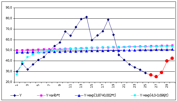

Приложение № 27
Polynomial Regression Analysis
-----------------------------------------------------------------------------
Dependent variable: Y
-----------------------------------------------------------------------------
Standard T
Parameter Estimate Error Statistic P-Value
-----------------------------------------------------------------------------
CONSTANT 37,8089 6,4945 5,82168 0,0000
t -6,05758 2,80081 -2,16279 0,0403
t^2 1,81869 0,359059 5,06515 0,0000
t^3 -0,114605 0,0172693 -6,63633 0,0000
t^4 0,00203425 0,000276526 7,35644 0,0000
-----------------------------------------------------------------------------
Analysis of Variance
-----------------------------------------------------------------------------
Source Sum of Squares Df Mean Square F-Ratio P-Value
-----------------------------------------------------------------------------
Model 7945,15 4 1986,29 60,19 0,0000
Residual 825,073 25 33,0029
-----------------------------------------------------------------------------
Total (Corr.) 8770,23 29
R-squared = 90,5923 percent
R-squared (adjusted for d.f.) = 89,0871 percent
Standard Error of Est. = 5,74482
Mean absolute error = 3,80267
Durbin-Watson statistic = 1,70505
The StatAdvisor
---------------
The output shows the results of fitting a fourth order polynomial
model to describe the relationship between Y and t. The equation of
the fitted model is
Y = 37,8089-6,05758*t + 1,81869*t^2-0,114605*t^3 + 0,00203425*t^4
95,0% confidence intervals for coefficient estimates
-----------------------------------------------------------------------------
Standard
Parameter Estimate Error Lower Limit Upper Limit
-----------------------------------------------------------------------------
CONSTANT 37,8089 6,4945 24,4332 51,1846
t -6,05758 2,80081 -11,826 -0,289188
t^2 1,81869 0,359059 1,07919 2,55818
t^3 -0,114605 0,0172693 -0,150172 -0,0790381
t^4 0,00203425 0,000276526 0,00146473 0,00260376
-----------------------------------------------------------------------------
The StatAdvisor
---------------
This table shows 95,0% confidence intervals for the coefficients in
the model. Confidence intervals show how precisely the coefficients
can be estimated given the amount of available data and the noise
which is present.
Predicted Values
------------------------------------------------------------------------------
95,00% 95,00%
Predicted Prediction Limits Confidence Limits
X Y Lower Upper Lower Upper
------------------------------------------------------------------------------
31,0 62,2508 44,3931 80,1085 48,8751 75,6265
------------------------------------------------------------------------------
The StatAdvisor
---------------
This table shows the predicted values for Y using the fitted model.
In addition to the best predictions, the table shows:
(1) 95,0% prediction intervals for new observations
(2) 95,0% confidence intervals for the mean of many observations
The prediction and confidence intervals correspond to the inner and
outer bounds on the graph of the fitted model.
П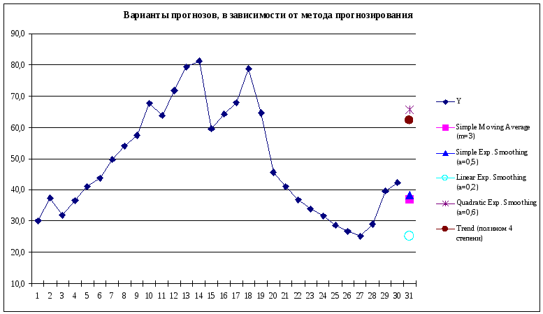 риложение
№28
риложение
№28
Приложение №29
|
t |
Y |
|
Абс. цеп. прирост Y |
Абс. цеп. прирост Yсгл (m=3) |
|
1 |
30,0 |
|
|
|
|
2 |
37,4 |
33,1 |
7,4 |
|
|
3 |
31,9 |
35,3 |
-5,5 |
2,2 |
|
4 |
36,7 |
36,5 |
4,8 |
1,2 |
|
5 |
41,0 |
40,5 |
4,3 |
3,9 |
|
6 |
43,7 |
44,8 |
2,7 |
4,3 |
|
7 |
49,7 |
49,1 |
6,0 |
4,3 |
|
8 |
53,9 |
53,7 |
4,2 |
4,6 |
|
9 |
57,4 |
59,6 |
3,5 |
6,0 |
|
10 |
67,6 |
63,0 |
10,2 |
3,3 |
|
11 |
63,9 |
67,8 |
-3,7 |
4,8 |
|
12 |
71,8 |
71,7 |
7,9 |
3,9 |
|
13 |
79,3 |
77,5 |
7,5 |
5,8 |
|
14 |
81,3 |
73,4 |
2,0 |
-4,1 |
|
15 |
59,6 |
68,4 |
-21,7 |
-5,0 |
|
16 |
64,2 |
63,9 |
4,6 |
-4,5 |
|
17 |
67,9 |
70,3 |
3,7 |
6,4 |
|
18 |
78,8 |
70,4 |
10,9 |
0,1 |
|
19 |
64,6 |
63,0 |
-14,2 |
-7,4 |
|
20 |
45,7 |
50,4 |
-18,9 |
-12,6 |
|
21 |
41,0 |
41,2 |
-4,7 |
-9,3 |
|
22 |
36,8 |
37,2 |
-4,2 |
-3,9 |
|
23 |
33,9 |
34,1 |
-2,9 |
-3,1 |
|
24 |
31,6 |
31,4 |
-2,3 |
-2,7 |
|
25 |
28,7 |
|
-2,9 |
|
|
26 |
26,7 |
|
|
|
|
27 |
25,1 |
|
|
|
|
28 |
29 |
|
|
|
|
29 |
39,7 |
|
|
|
|
30 |
42,4 |
|
|
|