Литература / The Scientist and Engineer's Guide to Digital Signal Processing (Steven W. Smith) / CH10

a single period. This forces the signal to spill over from one period into the adjacent periods. When the time domain is viewed as circular, portions of the signal that overflow on the right suddenly seem to reappear on the left side of the signal, and vice versa. That is, the overflowing portions of the signal alias themselves to a new location in the time domain. If this new location happens to already contain an existing signal, the whole mess adds, resulting in a loss of information. Circular convolution resulting from frequency domain multiplication (discussed in Chapter 9), is an excellent example of this type of aliasing.

Periodicity in the frequency domain behaves in much the same way, but is more complicated. Figure 10-9 shows an example. The upper figures show the magnitude and phase of the frequency spectrum, viewed as being composed of N /2 % 1 samples spread between 0 and 0.5 of the sampling rate. This is the simplest way of viewing the frequency spectrum, but it doesn't explain many of the DFT's properties.

The lower two figures show how the DFT views this frequency spectrum as being periodic. The key feature is that the frequency spectrum between 0 and 0.5 appears to have a mirror image of frequencies that run between 0 and -0.5. This mirror image of negative frequencies is slightly different for the magnitude and the phase signals. In the magnitude, the signal is flipped left- for-right. In the phase, the signal is flipped left-for-right, and changed in sign. As you recall, these two types of symmetry are given names: the magnitude is said to be an even signal (it has even symmetry), while the phase is said to be an odd signal (it has odd symmetry). If the frequency spectrum is converted into the real and imaginary parts, the real part will always be even, while the imaginary part will always be odd.

Taking these negative frequencies into account, the DFT views the frequency domain as periodic, with a period of 1.0 times the sampling rate, such as -0.5 to 0.5, or 0 to 1.0. In terms of sample numbers, this makes the length of the frequency domain period equal to N, the same as in the time domain.

The periodicity of the frequency domain makes it susceptible to frequency domain aliasing, completely analogous to the previously described time domain aliasing. Imagine a time domain signal that corresponds to some frequency spectrum. If the time domain signal is modified, it is obvious that the frequency spectrum will also be changed. If the modified frequency spectrum cannot fit in the space provided, it will push into the adjacent periods. Just as before, this aliasing causes two problems: frequencies aren't where they should be, and overlapping frequencies from different periods add, destroying information.

Frequency domain aliasing is more difficult to understand than time domain aliasing, since the periodic pattern is more complicated in the frequency domain. Consider a single frequency that is being forced to move from 0.01 to 0.49 in the frequency domain. The corresponding negative frequency is therefore moving from -0.01 to -0.49. When the positive frequency moves

across the 0.5 barrier, the negative frequency is pushed across the -0.5 barrier. Since the frequency domain is periodic, these same events are occurring in the other periods, such as between 0.5 and 1.5. A clone of the positive frequency is crossing frequency 1.5 from left to right, while a clone of the negative frequency is crossing 0.5 from right to left. Now imagine what this looks like if you can only see the frequency band of 0 to 0.5. It appears that a frequency leaving to the right, reappears on the right, but moving in the opposite direction.

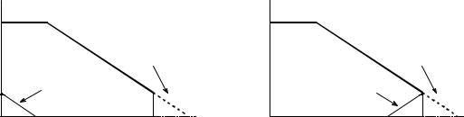
Figure 10-10 illustrates how aliasing appears in the time and frequency domains when only a single period is viewed. As shown in (a), if one end of a time domain signal is too long to fit inside a single period, the protruding end will be cut off and pasted onto the other side. In comparison, (b) shows that when a frequency domain signal overflows the period, the protruding end is folded over. Regardless of where the aliased segment ends up, it adds to whatever signal is already there, destroying information.

Let's take a closer look at these strange things called negative frequencies. Are they just some bizarre artifact of the mathematics, or do they have a real world meaning? Figure 10-11 shows what they are about. Figure (a) is a discrete signal composed of 32 samples. Imagine that you are given the task of finding the frequency spectrum that corresponds to these 32 points. To make your job easier, you are told that these points represent a discrete cosine wave. In other words, you must find the frequency and phase shift ( f and 2) such that x[n] ' cos(2Bn f / N % 2) matches the given samples. It isn't long before you come up with the solution shown in (b), that is, f ' 3 and 2 ' & B/4 .

If you stopped your analysis at this point, you only get 1/3 credit for the problem. This is because there are two other solutions that you have missed. As shown in (c), the second solution is f ' & 3 and 2 ' B/4 . Even if the idea of a negative frequency offends your sensibilities, it doesn't

FIGURE 10-10

Examples of aliasing in the time and frequency domains, when only a single period is considered. In the time domain, shown in (a), portions of the signal that exits to the right, reappear on the left. In the frequency domain, (b), portions of the signal that exit to the right, reappear on the right as if they had been folded over.

results in frequencies between 0 and -0.5. Lastly, the third solution makes up the infinite number of duplicated frequencies below -0.5 and above 0.5. If the signal we are analyzing is continuous, the first solution results in frequencies from zero to positive infinity, while the second solution results in frequencies from zero to negative infinity. The third group of solutions does not exist for continuous signals.

Many DSP techniques do not require the use of negative frequencies, or an understanding of the DFT's periodicity. For example, two common ones were described in the last chapter, spectral analysis, and the frequency response of systems. For these applications, it is completely sufficient to view the time domain as extending from sample 0 to N-1, and the frequency domain from zero to one-half of the sampling frequency. These techniques can use a simpler view of the world because they never result in portions of one period moving into another period. In these cases, looking at a single period is just as good as looking at the entire periodic signal.

However, certain procedures can only be analyzed by considering how signals overflow between periods. Two examples of this have already been presented, circular convolution and analog-to-digital conversion. In circular convolution, multiplication of the frequency spectra results in the time domain signals being convolved. If the resulting time domain signal is too long to fit inside a single period, it overflows into the adjacent periods, resulting in time domain aliasing. In contrast, analog-to-digital conversion is an example of frequency domain aliasing. A nonlinear action is taken in the time domain, that is, changing a continuous signal into a discrete signal by sampling. The problem is, the spectrum of the original analog signal may be too long to fit inside the discrete signal's spectrum. When we force the situation, the ends of the spectrum protrude into adjacent periods. Let's look at two more examples where the periodic nature of the DFT is important, compression & expansion of signals, and amplitude modulation.

Compression and Expansion, Multirate methods

As shown in Fig. 10-12, a compression of the signal in one domain results in an expansion in the other, and vice versa. For continuous signals, if X (f ) is the Fourier Transform of x( t ) , then 1/k × X( f / k ) is the Fourier Transform of x(k t), where k is the parameter controlling the expansion or contraction. If an event happens faster (it is compressed in time), it must be composed of higher frequencies. If an event happens slower (it is expanded in time), it must be composed of lower frequencies. This pattern holds if taken to either of the two extremes. That is, if the time domain signal is compressed so far that it becomes an impulse, the corresponding frequency spectrum is expanded so far that it becomes a constant value. Likewise, if the time domain is expanded until it becomes a constant value, the frequency domain becomes an impulse.

Discrete signals behave in a similar fashion, but there are a few more details. The first issue with discrete signals is aliasing . Imagine that the

time domain. Imagine that the frequency spectrum in (f) is compressed much harder, resulting in the time domain signal in (e) expanding into neighboring periods.

A second issue is to define exactly what it means to compress or expand a discrete signal. As shown in Fig. 10-12a, a discrete signal is compressed by compressing the underlying continuous curve that the samples lie on, and then resampling the new continuous curve to find the new discrete signal. Likewise, this same process for the expansion of discrete signals is shown in (e). When a discrete signal is compressed, events in the signal (such as the width of the pulse) happen over a fewer number of samples. Likewise, events in an expanded signal happen over a greater number of samples.

An equivalent way of looking at this procedure is to keep the underlying continuous waveform the same, but resample it at a different sampling rate. For instance, look at Fig. 10-13a, a discrete Gaussian waveform composed of 50 samples. In (b), the same underlying curve is represented by 400 samples. The change between (a) and (b) can be viewed in two ways: (1) the sampling rate has been kept constant, but the underlying waveform has been expanded to be eight times wider, or (2) the underlying waveform has been kept constant, but the sampling rate has increased by a factor of eight. Methods for changing the sampling rate in this way are called multirate techniques. If more samples are added, it is called interpolation. If fewer samples are used to represent the signal, it is called decimation. Chapter 3 describes how multirate techniques are used in ADC and DAC.

Here is the problem: if we are given an arbitrary discrete signal, how do we know what the underlying continuous curve is? It depends on if the signal's information is encoded in the time domain or in the frequency domain . For time domain encoded signals, we want the underlying continuous waveform to be a smooth curve that passes through all the samples. In the simplest case, we might draw straight lines between the points and then round the rough corners. The next level of sophistication is to use a curve fitting algorithm, such as a spline function or polynomial fit. There is not a single "correct" answer to this problem. This approach is based on minimizing irregularities in the time domain waveform, and completely ignores the frequency domain.

When a signal has information encoded in the frequency domain, we ignore the time domain waveform and concentrate on the frequency spectrum. As discussed in the last chapter, a finer sampling of a frequency spectrum (more samples between frequency 0 and 0.5) can be obtained by padding the time domain signal with zeros before taking the DFT. Duality allows this to work in the opposite direction. If we want a finer sampling in the time domain (interpolation), pad the frequency spectrum with zeros before taking the Inverse DFT. Say we want to interpolate a 50 sample signal into a 400 sample signal. It's done like this: (1) Take the 50 samples and add zeros to make the signal 64 samples long. (2) Use a 64 point DFT to find the frequency spectrum, which will consist of a 33 point real part and a 33 point imaginary part. (3) Pad the right side of the frequency spectrum

Multiplying Signals (Amplitude Modulation)

An important Fourier transform property is that convolution in one domain corresponds to multiplication in the other domain. One side of this was discussed in the last chapter: time domain signals can be convolved by multiplying their frequency spectra. Amplitude modulation is an example of the reverse situation, multiplication in the time domain corresponds to convolution in the frequency domain. In addition, amplitude modulation provides an excellent example of how the elusive negative frequencies enter into everyday science and engineering problems.

Audio signals are great for short distance communication; when you speak, someone across the room hears you. On the other hand, radio frequencies are very good at propagating long distances. For instance, if a 100 volt, 1 MHz sine wave is fed into an antenna, the resulting radio wave can be detected in the next room, the next country, and even on the next planet. Modulation is the process of merging two signals to form a third signal with desirable characteristics of both. This always involves nonlinear processes such as multiplication; you can't just add the two signals together. In radio communication, modulation results in radio signals that can propagate long distances and carry along audio or other information.

Radio communication is an extremely well developed discipline, and many modulation schemes have been developed. One of the simplest is called amplitude modulation. Figure 10-14 shows an example of how amplitude modulation appears in both the time and frequency domains. Continuous signals will be used in this example, since modulation is usually carried out in analog electronics. However, the whole procedure could be carried out in discrete form if needed (the shape of the future!).

Figure (a) shows an audio signal with a DC bias such that the signal always has a positive value. Figure (b) shows that its frequency spectrum is composed of frequencies from 300 Hz to 3 kHz, the range needed for voice communication, plus a spike for the DC component. All other frequencies have been removed by analog filtering. Figures (c) and (d) show the carrier wave, a pure sinusoid of much higher frequency than the audio signal. In the time domain, amplitude modulation consists of multiplying the audio signal by the carrier wave. As shown in (e), this results in an oscillatory waveform that has an instantaneous amplitude proportional to the original audio signal. In the jargon of the field, the envelope of the carrier wave is equal to the modulating signal. This signal can be routed to an antenna, converted into a radio wave, and then detected by a receiving antenna. This results in a signal identical to

(e) being generated in the radio receiver's electronics. A detector or demodulator circuit is then used to convert the waveform in (e) back into the waveform in (a).

Since the time domain signals are multiplied, the corresponding frequency spectra are convolved. That is, (f) is found by convolving (b) & (d). Since the spectrum of the carrier is a shifted delta function, the spectrum of the