

CHAPTER
Introduction to Digital Filters
14
Digital filters are used for two general purposes: (1) separation of signals that have been combined, and (2) restoration of signals that have been distorted in some way. Analog (electronic) filters can be used for these same tasks; however, digital filters can achieve far superior results. The most popular digital filters are described and compared in the next seven chapters. This introductory chapter describes the parameters you want to look for when learning about each of these filters.
Filter Basics
Digital filters are a very important part of DSP. In fact, their extraordinary performance is one of the key reasons that DSP has become so popular. As mentioned in the introduction, filters have two uses: signal separation and signal restoration. Signal separation is needed when a signal has been contaminated with interference, noise, or other signals. For example, imagine a device for measuring the electrical activity of a baby's heart (EKG) while still in the womb. The raw signal will likely be corrupted by the breathing and heartbeat of the mother. A filter might be used to separate these signals so that they can be individually analyzed.
Signal restoration is used when a signal has been distorted in some way. For example, an audio recording made with poor equipment may be filtered to better represent the sound as it actually occurred. Another example is the deblurring of an image acquired with an improperly focused lens, or a shaky camera.
These problems can be attacked with either analog or digital filters. Which is better? Analog filters are cheap, fast, and have a large dynamic range in both amplitude and frequency. Digital filters, in comparison, are vastly superior in the level of performance that can be achieved. For example, a low-pass digital filter presented in Chapter 16 has a gain of 1 +/- 0.0002 from DC to 1000 hertz, and a gain of less than 0.0002 for frequencies above
261
262 |
The Scientist and Engineer's Guide to Digital Signal Processing |
1001 hertz. The entire transition occurs within only 1 hertz. Don't expect this from an op amp circuit! Digital filters can achieve thousands of times better performance than analog filters. This makes a dramatic difference in how filtering problems are approached. With analog filters, the emphasis is on handling limitations of the electronics, such as the accuracy and stability of the resistors and capacitors. In comparison, digital filters are so good that the performance of the filter is frequently ignored. The emphasis shifts to the limitations of the signals, and the theoretical issues regarding their processing.
It is common in DSP to say that a filter's input and output signals are in the time domain. This is because signals are usually created by sampling at regular intervals of time. But this is not the only way sampling can take place. The second most common way of sampling is at equal intervals in space. For example, imagine taking simultaneous readings from an array of strain sensors mounted at one centimeter increments along the length of an aircraft wing. Many other domains are possible; however, time and space are by far the most common. When you see the term time domain in DSP, remember that it may actually refer to samples taken over time, or it may be a general reference to any domain that the samples are taken in.
As shown in Fig. 14-1, every linear filter has an impulse response, a step response and a frequency response. Each of these responses contains complete information about the filter, but in a different form. If one of the three is specified, the other two are fixed and can be directly calculated. All three of these representations are important, because they describe how the filter will react under different circumstances.
The most straightforward way to implement a digital filter is by convolving the input signal with the digital filter's impulse response. All possible linear filters can be made in this manner. (This should be obvious. If it isn't, you probably don't have the background to understand this section on filter design. Try reviewing the previous section on DSP fundamentals). When the impulse response is used in this way, filter designers give it a special name: the filter kernel.
There is also another way to make digital filters, called recursion. When a filter is implemented by convolution, each sample in the output is calculated by weighting the samples in the input, and adding them together. Recursive filters are an extension of this, using previously calculated values from the output, besides points from the input. Instead of using a filter kernel, recursive filters are defined by a set of recursion coefficients. This method will be discussed in detail in Chapter 19. For now, the important point is that all linear filters have an impulse response, even if you don't use it to implement the filter. To find the impulse response of a recursive filter, simply feed in an impulse, and see what comes out. The impulse responses of recursive filters are composed of sinusoids that exponentially decay in amplitude. In principle, this makes their impulse responses infinitely long. However, the amplitude eventually drops below the round-off noise of the system, and the remaining samples can be ignored. Because

Chapter 14Introduction to Digital Filters |
263 |
|
0.3 |
|
|
|
|
|
|
1.5 |
|
|
|
|
|
|
|
a. Impulse response |
|
|
|
|
|
c. Frequency response |
|
|
|||
Amplitude |
0.2 |
|
|
|
|
|
Amplitude |
1.0 |
|
|
|
|
|
0.1 |
|
|
|
|
FFT |
0.5 |
|
|
|
|
|
||
|
|
|
|
|
|
|
|
|
|
|
|||
|
|
|
|
|
|
|
|
|
|
|
|
||
|
0.0 |
|
|
|
|
|
|
0.0 |
|
|
|
|
|
|
-0.1 |
|
|
|
|
|
|
-0.5 |
|
|
|
|
|
|
0 |
32 |
64 |
96 |
1287 |
|
|
0 |
0.1 |
0.2 |
0.3 |
0.4 |
0.5 |
|
|
|
Sample number |
|
|
|
|
|
|
Frequency |
|
|
|
|
|
|
Integrate |
|
|
|
|
|
|
20 Log( |
) |
|
|
|
1.5 |
|
|
|
|
|
|
40 |
|
|
|
|
|
|
|
b. Step response |
|
|
|
|
|
d. Frequency response (in dB) |
|
||||
|
1.0 |
|
|
|
|
|
|
20 |
|
|
|
|
|
Amplitude |
|
|
|
|
|
Amplitude(dB) |
|
|
|
|
|
|
|
|
|
|
|
|
|
0 |
|
|
|
|
|
||
|
|
|
|
|
|
|
|
|
|
|
|
|
|
|
0.5 |
|
|
|
|
|
|
|
|
|
|
|
|
|
|
|
|
|
|
|
|
-20 |
|
|
|
|
|
|
0.0 |
|
|
|
|
|
|
-40 |
|
|
|
|
|
|
|
|
|
|
|
|
|
|
|
|
|
|
|
|
-0.5 |
|
|
|
|
|
|
-60 |
|
|
|
|
|
|
0 |
32 |
64 |
96 |
1287 |
|
|
0 |
0.1 |
0.2 |
0.3 |
0.4 |
0.5 |
|
|
|
Sample number |
|
|
|
|
|
|
Frequency |
|
|
|
FIGURE 14-1
Filter parameters. Every linear filter has an impulse response, a step response, and a frequency response. The step response, (b), can be found by discrete integration of the impulse response, (a). The frequency response can be found from the impulse response by using the Fast Fourier Transform (FFT), and can be displayed either on a linear scale, (c), or in decibels, (d).
of this characteristic, recursive filters are also called Infinite Impulse Response or IIR filters. In comparison, filters carried out by convolution are called Finite Impulse Response or FIR filters.
As you know, the impulse response is the output of a system when the input is an impulse. In this same manner, the step response is the output when the input is a step (also called an edge, and an edge response). Since the step is the integral of the impulse, the step response is the integral of the impulse response. This provides two ways to find the step response: (1) feed a step waveform into the filter and see what comes out, or (2) integrate the impulse response. (To be mathematically correct: integration is used with continuous signals, while discrete integration, i.e., a running sum, is used with discrete signals). The frequency response can be found by taking the DFT (using the FFT algorithm) of the impulse response. This will be reviewed later in this

264 |
The Scientist and Engineer's Guide to Digital Signal Processing |
chapter. The frequency response can be plotted on a linear vertical axis, such as in (c), or on a logarithmic scale (decibels), as shown in (d). The linear scale is best at showing the passband ripple and roll-off, while the decibel scale is needed to show the stopband attenuation.
Don't remember decibels? Here is a quick review. A bel (in honor of Alexander Graham Bell) means that the power is changed by a factor of ten. For example, an electronic circuit that has 3 bels of amplification produces an output signal with 10 × 10 × 10 ' 1000 times the power of the input. A decibel (dB) is one-tenth of a bel. Therefore, the decibel values of: -20dB, -10dB, 0dB, 10dB & 20dB, mean the power ratios: 0.01, 0.1, 1, 10, & 100, respectively. In other words, every ten decibels mean that the power has changed by a factor of ten.
Here's the catch: you usually want to work with a signal's amplitude, not its power. For example, imagine an amplifier with 20dB of gain. By definition, this means that the power in the signal has increased by a factor of 100. Since amplitude is proportional to the square-root of power, the amplitude of the output is 10 times the amplitude of the input. While 20dB means a factor of 100 in power, it only means a factor of 10 in amplitude. Every twenty decibels mean that the amplitude has changed by a factor of ten. In equation form:
EQUATION 14-1
Definition of decibels. Decibels are a way of expressing a ratio between two signals. Ratios of power (P1 & P2) use a different equation from ratios of amplitude (A1 & A2).
dB ' 10 log10 |
P2 |
|
P |
|
|
|
1 |
|
dB ' 20 log10 |
A2 |
|
|
|
|
A |
1 |
|
|
|
|
The above equations use the base 10 logarithm; however, many computer languages only provide a function for the base e logarithm (the natural log, written loge x or ln x ). The natural log can be use by modifying the above equations: dB ' 4.342945 loge (P2 / P1) and dB ' 8.685890 loge (A2 / A1).
Since decibels are a way of expressing the ratio between two signals, they are ideal for describing the gain of a system, i.e., the ratio between the output and the input signal. However, engineers also use decibels to specify the amplitude (or power) of a single signal, by referencing it to some standard. For example, the term: dBV means that the signal is being referenced to a 1 volt rms signal. Likewise, dBm indicates a reference signal producing 1 mW into a 600 ohms load (about 0.78 volts rms).
If you understand nothing else about decibels, remember two things: First, -3dB means that the amplitude is reduced to 0.707 (and the power is
Chapter 14Introduction to Digital Filters |
265 |
therefore reduced to 0.5). Second, memorize the following conversions between decibels and amplitude ratios:
60dB = 1000 40dB = 100 20dB = 10
0dB = 1 -20dB = 0.1 -40dB = 0.01 -60dB = 0.001
How Information is Represented in Signals
The most important part of any DSP task is understanding how information is contained in the signals you are working with. There are many ways that information can be contained in a signal. This is especially true if the signal is manmade. For instance, consider all of the modulation schemes that have been devised: AM, FM, single-sideband, pulse-code modulation, pulse-width modulation, etc. The list goes on and on. Fortunately, there are only two ways that are common for information to be represented in naturally occurring signals. We will call these: information represented in the time domain, and information represented in the frequency domain.
Information represented in the time domain describes when something occurs and what the amplitude of the occurrence is. For example, imagine an experiment to study the light output from the sun. The light output is measured and recorded once each second. Each sample in the signal indicates what is happening at that instant, and the level of the event. If a solar flare occurs, the signal directly provides information on the time it occurred, the duration, the development over time, etc. Each sample contains information that is interpretable without reference to any other sample. Even if you have only one sample from this signal, you still know something about what you are measuring. This is the simplest way for information to be contained in a signal.
In contrast, information represented in the frequency domain is more indirect. Many things in our universe show periodic motion. For example, a wine glass struck with a fingernail will vibrate, producing a ringing sound; the pendulum of a grandfather clock swings back and forth; stars and planets rotate on their axis and revolve around each other, and so forth. By measuring the frequency, phase, and amplitude of this periodic motion, information can often be obtained about the system producing the motion. Suppose we sample the sound produced by the ringing wine glass. The fundamental frequency and harmonics of the periodic vibration relate to the mass and elasticity of the material. A single sample, in itself, contains no information about the periodic motion, and therefore no information about the wine glass. The information is contained in the relationship between many points in the signal.
266 |
The Scientist and Engineer's Guide to Digital Signal Processing |
This brings us to the importance of the step and frequency responses. The step response describes how information represented in the time domain is being modified by the system. In contrast, the frequency response shows how information represented in the frequency domain is being changed. This distinction is absolutely critical in filter design because it is not possible to optimize a filter for both applications. Good performance in the time domain results in poor performance in the frequency domain, and vice versa. If you are designing a filter to remove noise from an EKG signal (information represented in the time domain), the step response is the important parameter, and the frequency response is of little concern. If your task is to design a digital filter for a hearing aid (with the information in the frequency domain), the frequency response is all important, while the step response doesn't matter. Now let's look at what makes a filter optimal for time domain or frequency domain applications.
Time Domain Parameters
It may not be obvious why the step response is of such concern in time domain filters. You may be wondering why the impulse response isn't the important parameter. The answer lies in the way that the human mind understands and processes information. Remember that the step, impulse and frequency responses all contain identical information, just in different arrangements. The step response is useful in time domain analysis because it matches the way humans view the information contained in the signals.
For example, suppose you are given a signal of some unknown origin and asked to analyze it. The first thing you will do is divide the signal into regions of similar characteristics. You can't stop from doing this; your mind will do it automatically. Some of the regions may be smooth; others may have large amplitude peaks; others may be noisy. This segmentation is accomplished by identifying the points that separate the regions. This is where the step function comes in. The step function is the purest way of representing a division between two dissimilar regions. It can mark when an event starts, or when an event ends. It tells you that whatever is on the left is somehow different from whatever is on the right. This is how the human mind views time domain information: a group of step functions dividing the information into regions of similar characteristics. The step response, in turn, is important because it describes how the dividing lines are being modified by the filter.
The step response parameters that are important in filter design are shown in Fig. 14-2. To distinguish events in a signal, the duration of the step response must be shorter than the spacing of the events. This dictates that the step response should be as fast (the DSP jargon) as possible. This is shown in Figs. (a) & (b). The most common way to specify the risetime (more jargon) is to quote the number of samples between the 10% and 90% amplitude levels. Why isn't a very fast risetime always possible? There are many reasons, noise reduction, inherent limitations of the data acquisition system, avoiding aliasing, etc.
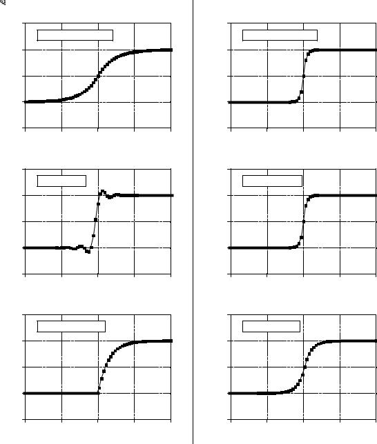
Chapter 14Introduction to Digital Filters |
267 |
|
|
|
POOR |
|
|
|
|
|
GOOD |
|
|
|
1.5 |
|
|
|
|
|
1.5 |
|
|
|
|
|
|
a. Slow step response |
|
|
|
|
b. Fast step response |
|
|
||
|
1.0 |
|
|
|
|
|
1.0 |
|
|
|
|
Amplitude |
0.5 |
|
|
|
|
Amplitude |
0.5 |
|
|
|
|
|
|
|
|
|
|
|
|
|
|
||
|
0.0 |
|
|
|
|
|
0.0 |
|
|
|
|
|
-0.5 |
|
|
|
|
|
-0.5 |
|
|
|
|
|
0 |
16 |
32 |
48 |
64 |
|
0 |
16 |
32 |
48 |
64 |
|
|
|
Sample number |
|
|
|
|
|
Sample number |
|
|
|
1.5 |
|
|
|
|
|
1.5 |
|
|
|
|
|
|
c. Overshoot |
|
|
|
|
d. No overshoot |
|
|
||
|
1.0 |
|
|
|
|
|
1.0 |
|
|
|
|
Amplitude |
0.5 |
|
|
|
|
Amplitude |
0.5 |
|
|
|
|
|
|
|
|
|
|
|
|
|
|
||
|
0.0 |
|
|
|
|
|
0.0 |
|
|
|
|
|
-0.5 |
|
|
|
|
|
-0.5 |
|
|
|
|
|
0 |
16 |
32 |
48 |
64 |
|
0 |
16 |
32 |
48 |
64 |
|
|
|
Sample number |
|
|
|
|
|
Sample number |
|
|
|
1.5 |
|
|
|
|
|
1.5 |
|
|
|
|
|
|
e. Nonlinear phase |
|
|
|
|
f. Linear phase |
|
|
||
|
1.0 |
|
|
|
|
|
1.0 |
|
|
|
|
Amplitude |
0.5 |
|
|
|
|
Amplitude |
0.5 |
|
|
|
|
|
|
|
|
|
|
|
|
|
|
||
|
0.0 |
|
|
|
|
|
0.0 |
|
|
|
|
|
-0.5 |
|
|
|
|
|
-0.5 |
|
|
|
|
|
0 |
16 |
32 |
48 |
64 |
|
0 |
16 |
32 |
48 |
64 |
|
|
|
Sample number |
|
|
|
|
|
Sample number |
|
|
FIGURE 14-2
Parameters for evaluating time domain performance. The step response is used to measure how well a filter performs in the time domain. Three parameters are important: (1) transition speed (risetime), shown in (a) and (b), (2) overshoot, shown in (c) and (d), and (3) phase linearity (symmetry between the top and bottom halves of the step), shown in (e) and (f).
Figures (c) and (d) shows the next parameter that is important: overshoot in the step response. Overshoot must generally be eliminated because it changes the amplitude of samples in the signal; this is a basic distortion of the information contained in the time domain. This can be summed up in
268 |
The Scientist and Engineer's Guide to Digital Signal Processing |
one question: Is the overshoot you observe in a signal coming from the thing you are trying to measure, or from the filter you have used?
Finally, it is often desired that the upper half of the step response be symmetrical with the lower half, as illustrated in (e) and (f). This symmetry is needed to make the rising edges look the same as the falling edges. This symmetry is called linear phase, because the frequency response has a phase that is a straight line (discussed in Chapter 19). Make sure you understand these three parameters; they are the key to evaluating time domain filters.
Frequency Domain Parameters
Figure 14-3 shows the four basic frequency responses. The purpose of these filters is to allow some frequencies to pass unaltered, while completely blocking other frequencies. The passband refers to those frequencies that are passed, while the stopband contains those frequencies that are blocked. The transition band is between. A fast roll-off means that the transition band is very narrow. The division between the passband and transition band is called the cutoff frequency. In analog filter design, the cutoff frequency is usually defined to be where the amplitude is reduced to 0.707 (i.e., -3dB). Digital filters are less standardized, and it is common to see 99%, 90%, 70.7%, and 50% amplitude levels defined to be the cutoff frequency.
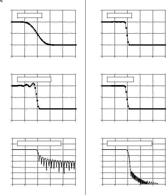
Figure 14-4 shows three parameters that measure how well a filter performs in the frequency domain. To separate closely spaced frequencies, the filter must have a fast roll-off, as illustrated in (a) and (b). For the passband frequencies to move through the filter unaltered, there must be no passband ripple, as shown in (c) and (d). Lastly, to adequately block the stopband frequencies, it is necessary to have good stopband attenuation, displayed in (e) and (f).
FIGURE 14-3
The four common frequency responses. Frequency domain filters are generally used to pass certain frequencies (the passband), while blocking others (the stopband). Four responses are the most common: low-pass, high-pass, band-pass, and band-reject.
|
a. Low-pass |
|
Amplitude |
passband |
transition |
|
band |
|
|
|
|
|
|
stopband |
|
|
Frequency |
|
b. High-pass |
|
Amplitude |
|
|
Frequency
Amplitude

Amplitude

c. Band-pass
Frequency
d. Band-reject
Frequency
Chapter 14Introduction to Digital Filters |
269 |
|
|
|
POOR |
|
|
|
|
|
GOOD |
|
|
||
|
1.5 |
|
|
|
|
|
|
1.5 |
|
|
|
|
|
|
a. |
Slow roll-off |
|
|
|
|
|
b. Fast roll-off |
|
|
|
||
Amplitude |
1.0 |
|
|
|
|
|
Amplitude |
1.0 |
|
|
|
|
|
0.5 |
|
|
|
|
|
0.5 |
|
|
|
|
|
||
|
|
|
|
|
|
|
|
|
|
|
|
||
|
0.0 |
|
|
|
|
|
|
0.0 |
|
|
|
|
|
|
-0.5 |
|
|
|
|
|
|
-0.5 |
|
|
|
|
|
|
0 |
0.1 |
0.2 |
0.3 |
0.4 |
0.5 |
|
0 |
0.1 |
0.2 |
0.3 |
0.4 |
0.5 |
|
|
|
Frequency |
|
|
|
|
|
Frequency |
|
|
||
|
1.5 |
|
|
|
|
|
|
1.5 |
|
|
|
|
|
|
c. Ripple in passband |
|
|
|
|
|
d. Flat passband |
|
|
|
|||
1.0 |
1.0 |
Amplitude |
0.5 |
|
|
|
|
|
Amplitude |
0.5 |
|
|
|
|
|
|
|
|
|
|
|
|
|
|
|
|
|
||
|
0.0 |
|
|
|
|
|
|
0.0 |
|
|
|
|
|
|
-0.5 |
|
|
|
|
|
|
-0.5 |
|
|
|
|
|
|
0 |
0.1 |
0.2 |
0.3 |
0.4 |
0.5 |
|
0 |
0.1 |
0.2 |
0.3 |
0.4 |
0.5 |
|
|
|
Frequency |
|
|
|
|
|
Frequency |
|
|
||
|
40 |
|
|
|
|
|
|
40 |
|
|
|
|
|
|
20 |
e. Poor stopband attenuation |
|
|
|
20 |
f. Good stopband attenuation |
|
|
||||
(dB) |
0 |
|
|
|
|
|
(dB) |
0 |
|
|
|
|
|
-20 |
|
|
|
|
|
-20 |
|
|
|
|
|
||
Amplitude |
|
|
|
|
|
Amplitude |
|
|
|
|
|
||
-40 |
|
|
|
|
|
-40 |
|
|
|
|
|
||
|
|
|
|
|
|
|
|
|
|
|
|
||
|
-60 |
|
|
|
|
|
|
-60 |
|
|
|
|
|
|
-80 |
|
|
|
|
|
|
-80 |
|
|
|
|
|
|
-100 |
|
|
|
|
|
|
-100 |
|
|
|
|
|
|
-120 |
|
|
|
|
|
|
-120 |
|
|
|
|
|
|
0 |
0.1 |
0.2 |
0.3 |
0.4 |
0.5 |
|
0 |
0.1 |
0.2 |
0.3 |
0.4 |
0.5 |
|
|
|
Frequency |
|
|
|
|
|
Frequency |
|
|
||
FIGURE 14-4
Parameters for evaluating frequency domain performance. The frequency responses shown are for low-pass filters. Three parameters are important: (1) roll-off sharpness, shown in (a) and (b), (2) passband ripple, shown in (c) and (d), and (3) stopband attenuation, shown in (e) and (f).
Why is there nothing about the phase in these parameters? First, the phase isn't important in most frequency domain applications. For example, the phase of an audio signal is almost completely random, and contains little useful information. Second, if the phase is important, it is very easy to make digital
270 |
The Scientist and Engineer's Guide to Digital Signal Processing |
filters with a perfect phase response, i.e., all frequencies pass through the filter with a zero phase shift (also discussed in Chapter 19). In comparison, analog filters are ghastly in this respect.
Previous chapters have described how the DFT converts a system's impulse response into its frequency response. Here is a brief review. The quickest way to calculate the DFT is by means of the FFT algorithm presented in Chapter 12. Starting with a filter kernel N samples long, the FFT calculates the frequency spectrum consisting of an N point real part and an N point imaginary part. Only samples 0 to N/2 of the FFT's real and imaginary parts contain useful information; the remaining points are duplicates (negative frequencies) and can be ignored. Since the real and imaginary parts are difficult for humans to understand, they are usually converted into polar notation as described in Chapter 8. This provides the magnitude and phase signals, each running from sample 0 to sample N/2 (i.e., N/2 %1 samples in each signal). For example, an impulse response of 256 points will result in a frequency response running from point 0 to 128. Sample 0 represents DC, i.e., zero frequency. Sample 128 represents one-half of the sampling rate. Remember, no frequencies higher than one-half of the sampling rate can appear in sampled data.
The number of samples used to represent the impulse response can be arbitrarily large. For instance, suppose you want to find the frequency response of a filter kernel that consists of 80 points. Since the FFT only works with signals that are a power of two, you need to add 48 zeros to the signal to bring it to a length of 128 samples. This padding with zeros does not change the impulse response. To understand why this is so, think about what happens to these added zeros when the input signal is convolved with the system's impulse response. The added zeros simply vanish in the convolution, and do not affect the outcome.
Taking this a step further, you could add many zeros to the impulse response to make it, say, 256, 512, or 1024 points long. The important idea is that longer impulse responses result in a closer spacing of the data points in the frequency response. That is, there are more samples spread between DC and one-half of the sampling rate. Taking this to the extreme, if the impulse response is padded with an infinite number of zeros, the data points in the frequency response are infinitesimally close together, i.e., a continuous line. In other words, the frequency response of a filter is really a continuous signal between DC and one-half of the sampling rate. The output of the DFT is a sampling of this continuous line. What length of impulse response should you use when calculating a filter's frequency response? As a first thought, try N '1024 , but don't be afraid to change it if needed (such as insufficient resolution or excessive computation time).
Keep in mind that the "good" and "bad" parameters discussed in this chapter are only generalizations. Many signals don't fall neatly into categories. For example, consider an EKG signal contaminated with 60 hertz interference. The information is encoded in the time domain, but the interference is best dealt with in the frequency domain. The best design for this application is