Литература / The Scientist and Engineer's Guide to Digital Signal Processing (Steven W. Smith) / CH13

FIGURE 13-8

Example of the Fourier Transform. The time domain signal, x(t ), extends from negative to positive infinity. The frequency domain is composed of a real part, Re X(T) , and an imaginary part, Im X(T), each extending from zero to positive infinity. The frequency axis in this illustration is labeled in cycles per second (hertz). To convert to natural frequency, multiply the numbers on the frequency axis by 2B.

Greek omega. As you recall, this notation is called the natural frequency, and has the units of radians per second. That is, T' 2Bf , where f is the frequency in cycles per second (hertz). The natural frequency notation is favored by mathematicians and others doing signal processing by solving equations, because there are usually fewer symbols to write.

The analysis equations for continuous signals follow the same strategy as the discrete case: correlation with sine and cosine waves. The equations are:

& 4

As an example of using the analysis equations, we will find the frequency response of the RC low-pass filter. This is done by taking the Fourier transform of its impulse response, previously shown in Fig. 13-4, and described by:

The frequency response is found by plugging the impulse response into the analysis equations. First, the real part:

"2

Re H (T) '

"2 % T2

Using this same approach, the imaginary part of the frequency response is calculated to be:

& T"

Im H (T) '

"2 % T2

Just as with discrete signals, the rectangular representation of the frequency domain is great for mathematical manipulation, but difficult for human understanding. The situation can be remedied by converting into polar notation with the standard relations: Mag H (T) ' [ Re H (T)2 % Im H (T)2 ]½ and Phase H(T) ' arctan [ Re H(T) / Im H(T)] . Working through the algebra

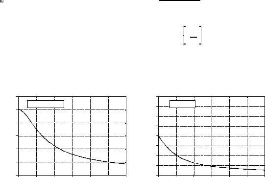
provides the frequency response of the RC low-pass filter as magnitude and phase (i.e., polar form):

"

Mag H (T) '

[ "2 % T2 ]1/2

Phase H (T) ' arctan & T

"

Figure 13-9 shows graphs of these curves for a cutoff frequency of 1000 hertz (i.e., "' 2B1000 ).

FIGURE 13-9

Frequency response of an RC low-pass filter. These curves were derived by calculating the Fourier transform of the impulse response, and then converting to polar form.

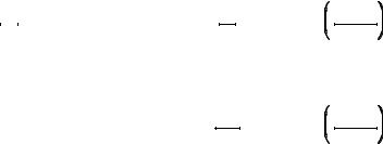
The Fourier Series

This brings us to the last member of the Fourier transform family: the Fourier series. The time domain signal used in the Fourier series is periodic and continuous. Figure 13-10 shows several examples of continuous waveforms that repeat themselves from negative to positive infinity. Chapter 11 showed that periodic signals have a frequency spectrum consisting of harmonics. For instance, if the time domain repeats at 1000 hertz (a period of 1 millisecond), the frequency spectrum will contain a first harmonic at 1000 hertz, a second harmonic at 2000 hertz, a third harmonic at 3000 hertz, and so forth. The first harmonic, i.e., the frequency that the time domain repeats itself, is also called the fundamental frequency. This means that the frequency spectrum can be viewed in two ways: (1) the frequency spectrum is continuous, but zero at all frequencies except the harmonics, or (2) the frequency spectrum is discrete, and only defined at the harmonic frequencies. In other words, the frequencies between the harmonics can be thought of as having a value of zero, or simply

256 The Scientist and Engineer's Guide to Digital Signal Processing

not existing. The important point is that they do not contribute to forming the time domain signal.

The Fourier series synthesis equation creates a continuous periodic signal with a fundamental frequency, f, by adding scaled cosine and sine waves with frequencies: f, 2f, 3f, 4f, etc. The amplitudes of the cosine waves are held in the variables: a1, a2, a3, a4, etc., while the amplitudes of the sine waves are held in: b1, b2, b3, b4, and so on. In other words, the "a" and "b" coefficients are the real and imaginary parts of the frequency spectrum, respectively. In addition, the coefficient a0 is used to hold the DC value of the time domain waveform. This can be viewed as the amplitude of a cosine wave with zero frequency (a constant value). Sometimes a0 is grouped with the other "a" coefficients, but it is often handled separately because it requires special calculations. There is no b0 coefficient since a sine wave of zero frequency has a constant value of zero, and would be quite useless. The synthesis equation is written:

The corresponding analysis equations for the Fourier series are usually written in terms of the period of the waveform, denoted by T, rather than the fundamental frequency, f (where f ' 1/T ). Since the time domain signal is periodic, the sine and cosine wave correlation only needs to be evaluated over a single period, i.e., & T /2 to T /2 , 0 to T, -T to 0, etc. Selecting different limits makes the mathematics different, but the final answer is always the same. The Fourier series analysis equations are:

FIGURE 13-10

Examples of the Fourier series. Six common time domain waveforms are shown, along with the equations to calculate their "a" and "b" coefficients.

Time

FIGURE 13-11

Example of calculating a Fourier series. This is a pulse train with a duty cycle of d = k/T. The Fourier series coefficients are calculated by correlating the waveform with cosine and sine waves over any full period. In this example, the period from -T/2 to T/2 is used.

Figure 13-11 shows an example of calculating a Fourier series using these equations. The time domain signal being analyzed is a pulse train, a square wave with unequal high and low durations. Over a single period from & T /2 to T /2 , the waveform is given by:

The duty cycle of the waveform (the fraction of time that the pulse is "high") is thus given by d ' k /T . The Fourier series coefficients can be found by evaluating Eq. 13-5. First, we will find the DC component, a0 :

T/2

This result should make intuitive sense; the DC component is simply the average value of the signal. A similar analysis provides the "a" coefficients:

The "b" coefficients are calculated in this same way; however, they all turn out to be zero. In other words, this waveform can be constructed using only cosine waves, with no sine waves being needed.

The "a" and "b" coefficients will change if the time domain waveform is shifted left or right. For instance, the "b" coefficients in this example will be zero only if one of the pulses is centered on t ' 0 . Think about it this way. If the waveform is even (i.e., symmetrical around t ' 0 ), it will be composed solely of even sinusoids, that is, cosine waves. This makes all of the "b" coefficients equal to zero. If the waveform if odd (i.e., symmetrical but opposite in sign around t ' 0 ), it will be composed of odd sinusoids, i.e., sine waves. This results in the "a" coefficients being zero. If the coefficients are converted to polar notation (say, Mn and 2n coefficients), a shift in the time domain leaves the magnitude unchanged, but adds a linear component to the phase.

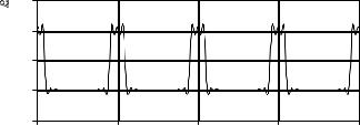
To complete this example, imagine a pulse train existing in an electronic circuit, with a frequency of 1 kHz, an amplitude of one volt, and a duty cycle of 0.2. The table in Fig. 13-12 provides the amplitude of each harmonic contained in this waveform. Figure 13-12 also shows the synthesis of the waveform using only the first fourteen of these harmonics. Even with this number of harmonics, the reconstruction is not very good. In mathematical jargon, the Fourier series converges very slowly. This is just another way of saying that sharp edges in the time domain waveform results in very high frequencies in the spectrum. Lastly, be sure and notice the overshoot at the sharp edges, i.e., the Gibbs effect discussed in Chapter 11.

An important application of the Fourier series is electronic frequency multiplication. Suppose you want to construct a very stable sine wave oscillator at 150 MHz. This might be needed, for example, in a radio

transmitter operating at this frequency. High stability calls for the circuit to be crystal controlled. That is, the frequency of the oscillator is determined by a resonating quartz crystal that is a part of the circuit. The problem is, quartz crystals only work to about 10 MHz. The solution is to build a crystal controlled oscillator operating somewhere between 1 and 10 MHz, and then multiply the frequency to whatever you need. This is accomplished by distorting the sine wave, such as by clipping the peaks with a diode, or running the waveform through a squaring circuit. The harmonics in the distorted waveform are then isolated with band-pass filters. This allows the frequency to be doubled, tripled, or multiplied by even higher integers numbers. The most common technique is to use sequential stages of doublers and triplers to generate the required frequency multiplication, rather than just a single stage. The Fourier series is important to this type of design because it describes the amplitude of the multiplied signal, depending on the type of distortion and harmonic selected.