Data-Structures-And-Algorithms-Alfred-V-Aho

Data Structures and Algorithms: CHAPTER 3: Trees

example, by numbering the children of each node after numbering the parent, and numbering the children in

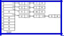
procedure NPREORDER ( T: TREE );

{ nonrecursive preorder traversal of tree T }

var

m: node; { a temporary }

S: STACK; { stack of nodes holding path from the root to the parent TOP(S) of the "current" node m }

begin

{ initialize } MAKENULL(S); m := ROOT(T);

while true do

if m < > Λ then begin print(LABEL(m, T)); PUSH(m, S);

{ explore leftmost child of m } m := LEFTMOST_CHILD(m, T)

end

else begin

{ exploration of path on stack is now complete }

if EMPTY(S) then return;

{explore right sibling of node on top of stack }

m := RIGHT_SIBLING(TOP(S), T); POP(S)

end

end; { NPREORDER }

Fig. 3.9. A nonrecursive preorder procedure.

increasing order from left to right. On that assumption, we have written the function RIGHT_SIBLING in Fig. 3.11, for types node and TREE that are defined as follows:

type

http://www.ourstillwaters.org/stillwaters/csteaching/DataStructuresAndAlgorithms/mf1203.htm (11 of 32) [1.7.2001 19:01:17]

Data Structures and Algorithms: CHAPTER 3: Trees

node = integer;

TREE = array [1..maxnodes] of node;

For this implementation we assume the null node Λ is represented by 0.

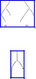
Fig. 3.10. A tree and its parent pointer representation.

function RIGHT_SIBLING ( n: node; T: TREE ): node; { return the right sibling of node n in tree T }

var

i, parent: node; begin

parent: = T[n];

for i := n + 1 to maxnodes do

{ search for node after n with same parent } if T[i] = parent then

return (i);

return (0) { null node will be returned if no right sibling is ever found }

end; { RIGHT_SIBLING }

Fig. 3.11. Right sibling operation using array representation.

Representation of Trees by Lists of Children

An important and useful way of representing trees is to form for each node a list of its children. The lists can be represented by any of the methods suggested in Chapter 2, but because the number of children each node may have can be variable, the linked-list representations are often more appropriate.

Figure 3.12 suggests how the tree of Fig. 3.10(a) might be represented. There is an array of header cells, indexed by nodes, which we assume to be numbered 1, 2, . .

http://www.ourstillwaters.org/stillwaters/csteaching/DataStructuresAndAlgorithms/mf1203.htm (12 of 32) [1.7.2001 19:01:17]

Data Structures and Algorithms: CHAPTER 3: Trees

. , 10. Each header points to a linked list of "elements," which are nodes. The elements on the list headed by header[i] are the children of node i; for example, 9 and 10 are the children of 3.

Fig. 3.12. A linked-list representation of a tree.

Let us first develop the data structures we need in terms of an abstract data type LIST (of nodes), and then give a particular implementation of lists and see how the abstractions fit together. Later, we shall see some of the simplifications we can make. We begin with the following type declarations:

type

node = integer;

LIST = { appropriate definition for list of nodes }; position = { appropriate definition for positions in lists }; TREE = record

header: array [1..maxnodes] of LIST; labels: array [1..maxnodes] of labeltype; root: node

end;

We assume that the root of each tree is stored explicitly in the root field. Also, 0 is used to represent the null node.

Figure 3.13 shows the code for the LEFTMOST_CHILD operation. The reader should write the code for the other operations as exercises.

function LEFTMOST_CHILD ( n: node; T: TREE ): node; { returns the leftmost child of node n of tree T }

var

L: LIST; { shorthand for the list of n's children } begin

L := T.header[n];

if EMPTY(L) then { n is a leaf } return (0)

http://www.ourstillwaters.org/stillwaters/csteaching/DataStructuresAndAlgorithms/mf1203.htm (13 of 32) [1.7.2001 19:01:17]

Data Structures and Algorithms: CHAPTER 3: Trees

else

return (RETRIEVE(FIRST(L), L)) end; { LEFTMOST_CHILD }

Fig. 3.13. Function to find leftmost child.

Now let us choose a particular implementation of lists, in which both LIST and position are integers, used as cursors into an array cellspace of records:

var

cellspace : array [1..maxnodes] of record node: integer;

next: integer end;

To simplify, we shall not insist that lists of children have header cells. Rather, we shall let T.header [n] point directly to the first cell of the list, as is suggested by Fig. 3.12. Figure 3.14(a) shows the function LEFTMOST_CHILD of Fig. 3.13 rewritten for this specific implementation. Figure 3.14(b) shows the operator PARENT, which is more difficult to write using this representation of lists, since a search of all lists is required to determine on which list a given node appears.

The Leftmost-Child, Right-Sibling

Representation

The data structure described above has, among other shortcomings, the inability to create large trees from smaller ones, using the CREATEi operators. The reason is that, while all trees share cellspace for linked lists of children, each has its own array of headers for its nodes. For example, to implement CREATE2(v, T1, T2) we would have to copy T1 and T2 into a third tree and add a new node with label v and two children -- the roots of T1 and T2.

If we wish to build trees from smaller ones, it is best that the representation of nodes from all trees share one area. The logical extension of Fig. 3.12 is to replace the header array by an array nodespace consisting of records with

function LEFTMOST_CHILD ( n: node; T: TREE ): node;

http://www.ourstillwaters.org/stillwaters/csteaching/DataStructuresAndAlgorithms/mf1203.htm (14 of 32) [1.7.2001 19:01:17]

Data Structures and Algorithms: CHAPTER 3: Trees

{ returns the leftmost child of node n on tree T } var

L: integer; { a cursor to the beginning of the list of n's children } begin

L := T.header[n];

if L = 0 then { n is a leaf } return (0)

else

return (cellspace[L].node) end; { LEFTMOST_CHILD }

(a) The function LEFTMOST_CHILD.

function PARENT ( n: node; T: TREE ): node; { returns the parent of node n in tree T }

var

p: node; { runs through possible parents of n } i: position; { runs down list of p's children }

begin

for p := 1 to maxnodes do begin i := T.header[p];

while i <> 0 do { see if n is among children of

p }

if cellspace[i].node = n then return (p)

else

i := cellspace[i].next

end;

return (0) { return null node if parent not found } end; { PARENT }

(b) The function PARENT.

Fig. 3.14. Two functions using linked-list representation of trees.

two fields label and header. This array will hold headers for all nodes of all trees. Thus, we declare

var

nodespace : array [1..maxnodes] of record label: labeltype;

header: integer; { cursor to cellspace }

http://www.ourstillwaters.org/stillwaters/csteaching/DataStructuresAndAlgorithms/mf1203.htm (15 of 32) [1.7.2001 19:01:17]

Data Structures and Algorithms: CHAPTER 3: Trees

end;

Then, since nodes are no longer named 1, 2, . . . , n, but are represented by arbitrary indices in nodespace, it is no longer feasible for the field node of cellspace to represent the "number" of a node; rather, node is now a cursor into nodespace, indicating the position of that node. The type TREE is simply a cursor into nodespace, indicating the position of the root.

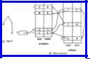
Example 3.7. Figure 3.15(a) shows a tree, and Fig. 3.15(b) shows the data structure where we have placed the nodes labeled A, B, C, and D arbitrarily in positions 10, 5, 11, and 2 of nodespace. We have also made arbitrary choices for the cells of cellspace used for lists of children.

Fig. 3.15. Another linked-list structure for trees.

The structure of Fig. 3.15(b) is adequate to merge trees by the CREATEi operations. This data structure can be significantly simplified, however, First, observe that the chains of next pointers in cellspace are really right-sibling pointers.

Using these pointers, we can obtain leftmost children as follows. Suppose cellspace[i].node = n. (Recall that the "name" of a node, as opposed to its label, is in effect its index in nodespace, which is what cellspace[i].node gives us.) Then nodespace[n].header indicates the cell for the leftmost child of n in cellspace, in the sense that the node field of that cell is the name of that node in nodespace.

We can simplify matters if we identify a node not with its index in nodespace, but with the index of the cell in cellspace that represents it as a child. Then, the next pointers of cellspace truly point to right siblings, and the information contained in the nodespace array can be held by introducing a field leftmost_child in cellspace. The datatype TREE becomes an integer used as a cursor to cellspace indicating the root of the tree. We declare cellspace to have the following structure.

var

cellspace : array [1..maxnodes] of record label: labeltype;

http://www.ourstillwaters.org/stillwaters/csteaching/DataStructuresAndAlgorithms/mf1203.htm (16 of 32) [1.7.2001 19:01:17]

Data Structures and Algorithms: CHAPTER 3: Trees

leftmost_child: integer; right_sibling: integer;

end;

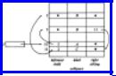
Example 3.8. The tree of Fig. 3.15(a) is represented in our new data structure in Fig. 3.16. The same arbitrary indices as in Fig. 3.15(b) have been used for the nodes.

Fig. 3.16. Leftmost-child, right-sibling representation of a tree.

All operations but PARENT are straightforward to implement in the leftmostchild, right-sibling representation. PARENT requires searching the entire cellspace. If we need to perform the PARENT operation efficiently, we can add a fourth field to cellspace to indicate the parent of a node directly.

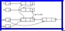
As an example of a tree operation written to use the leftmostchild, right-sibling structure as in Fig. 3.16, we give the function CREATE2 in Fig. 3.17. We assume that unused cells are linked in an available space list, headed by avail, and that available cells are linked by their right-sibling fields. Figure 3.18 shows the old (solid) and the new (dashed) pointers.

function CREATE2 ( v: labeltype; T1, T2: integer ): integer;

{ returns new tree with root v, having T1 and T2 as subtrees } var

temp: integer; { holds index of first available cell for root of new tree }

begin

temp := avail;

avail := cellspace [avail].right_sibling; cellspace[temp].leftmost_child := T1; cellspace[temp].label := v; cellspace[temp].right_sibling := 0; cellspace[T1].right_sibling := T2; cellspace[T2].right_sibling := 0; { not necessary;

that field should be 0 as the cell was formerly a root } return (temp)

http://www.ourstillwaters.org/stillwaters/csteaching/DataStructuresAndAlgorithms/mf1203.htm (17 of 32) [1.7.2001 19:01:17]

Data Structures and Algorithms: CHAPTER 3: Trees

end; { CREATE2 }

Fig. 3.17. The function CREATE2.

Fig. 3.18. Pointer changes produced by CREATE2.

Alternatively, we can use less space but more time if we put in the right-sibling field of the rightmost child a pointer to the parent, in place of the null pointer that would otherwise be there. To avoid confusion, we need a bit in every cell indicating whether the right-sibling field holds a pointer to the right sibling or to the parent.

Given a node, we find its parent by following right-sibling pointers until we find one that is a parent pointer. Since all siblings have the same parent, we thereby find our way to the parent of the node we started from. The time required to find a node's parent in this representation depends on the number of siblings a node has.

3.4 Binary Trees

The tree we defined in Section 3.1 is sometimes called an ordered, oriented tree because the children of each node are ordered from left-to-right, and because there is an oriented path (path in a particular direction) from every node to its descendants. Another useful, and quite different, notion of "tree" is the binary tree, which is either an empty tree, or a tree in which every node has either no children, a left child, a right child, or both a left and a right child. The fact that each child in a binary tree is designated as a left child or as a right child makes a binary tree different from the ordered, oriented tree of Section 3.1.

Example 3.9. If we adopt the convention that left children are drawn extending to the left, and right children to the right, then Fig. 3.19 (a) and (b) represent two different binary trees, even though both "look like" the ordinary (ordered, oriented) tree of Fig. 3.20. However, let us emphasize that Fig. 3.19(a) and (b) are not the same binary tree, nor are either in any sense equal to Fig. 3.20, for the simple reason that binary trees are not directly comparable with ordinary trees. For example, in Fig. 3.19(a), 2 is the left child of 1, and 1 has no right child, while in Fig. 3.19(b), 1 has no left child but has 2 as a right child. In either binary tree, 3 is the left child of 2, and 4 is 2's right child.

http://www.ourstillwaters.org/stillwaters/csteaching/DataStructuresAndAlgorithms/mf1203.htm (18 of 32) [1.7.2001 19:01:17]

Data Structures and Algorithms: CHAPTER 3: Trees

The preorder and postorder listings of a binary tree are similar to those of an ordinary tree given on p. 78. The inorder listing of the nodes of a binary tree with root n, left subtree T1 and right subtree T2 is the inorder listing of T1 followed by n followed by the inorder listing of T2. For example, 35241 is the inorder listing of the nodes of Fig. 3.19(a).

Representing Binary Trees

A convenient data structure for representing a binary tree is to name the nodes 1, 2, .

. . , n, and to use an array of records declared

var

cellspace : array [1..maxnodes] of record leftchild: integer;

rightchild: integer; end;

Fig. 3.19. Two binary trees.

Fig. 3.20. An "ordinary" tree.

The intention is that cellspace[i].leftchild is the left child of node i, and rightchild is analogous. A value of 0 in either field indicates the absence of a child.

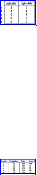
Example 3.10. The binary tree of Fig. 3.19(a) can be represented as shown in Fig. 3.21.

http://www.ourstillwaters.org/stillwaters/csteaching/DataStructuresAndAlgorithms/mf1203.htm (19 of 32) [1.7.2001 19:01:17]

Data Structures and Algorithms: CHAPTER 3: Trees

An Example: Huffman Codes

Let us give an example of how binary trees can be used as a data structure. The particular problem we shall consider is the construction of "Huffman codes." Suppose we have messages consisting of sequences of characters. In each message, the characters are independent and appear with a known

Fig. 3.21. Representation of a binary tree.

probability in any given position; the probabilities are the same for all positions. As an example, suppose we have a message made from the five characters a, b, c, d, e, which appear with probabilities .12, .4, .15, .08, .25, respectively.

We wish to encode each character into a sequence of 0's and 1's so that no code for a character is the prefix of the code for any other character. This prefix property allows us to decode a string of 0's and 1's by repeatedly deleting prefixes of the string that are codes for characters.

Example 3.11. Figure 3.22 shows two possible codes for our five symbol alphabet. Clearly Code 1 has the prefix property, since no sequence of three bits can be the prefix of another sequence of three bits. The decoding algorithm for Code 1 is simple. Just "grab" three bits at a time and translate each group of three into a character. Of course, sequences 101, 110, and 111 are impossible, if the string of bits really codes characters according to Code 1. For example, if we receive 001010011 we know the original message was bcd.

Fig. 3.22. Two binary codes.

It is easy to check that Code 2 also has the prefix property. We can decode a string of bits by repeatedly "grabbing" prefixes that are codes for characters and removing them, just as we did for Code 1. The only difference is that here, we cannot slice up the entire sequence of bits at once, because whether we take two or three bits

http://www.ourstillwaters.org/stillwaters/csteaching/DataStructuresAndAlgorithms/mf1203.htm (20 of 32) [1.7.2001 19:01:17]