

2
The Solow Growth Model
The previous chapter introduced a number of basic facts and posed the main questions concerning the sources of economic growth over time and the causes of differences in economic performance across countries. These questions are central not only to growth theory but also to macroeconomics and the social sciences more generally. Our next task is to develop a simple framework that can help us think about the proximate causes and the mechanics of the process of economic growth and cross-country income differences. We will use this framework both to study potential sources of economic growth and also to perform simple comparative statics to gain an understanding of which country characteristics are
conducive to higher levels of income per capita and more rapid economic growth.
Our starting point is the so-called Solow-Swan model named after Robert (Bob) Solow and Trevor Swan, or simply the Solow model, named after the more famous of the two economists. These economists published two pathbreaking articles in the same year, 1956 (Solow, 1956; Swan, 1956) introducing the Solow model. Bob Solow later developed many implications and applications of this model and was awarded the Nobel prize in economics for his contributions. This model has shaped the way we approach not only economic growth but also the entire field of macroeconomics. Consequently, a by-product of our analysis of this chapter is a detailed exposition of a workhorse model of macroeconomics.
The Solow model is remarkable in its simplicity. Looking at it today, one may fail to appreciate how much of an intellectual breakthrough it was. Before the advent of the Solow growth model, the most common approach to economic growth built on the model developed by Roy Harrod and Evsey Domar (Harrod, 1939; Domar, 1946). The Harrod-Domar model emphasized potential dysfunctional aspects of economic growth, for example, how economic growth could go hand-in-hand with increasing unemployment (see Exercise 2.23 on this model). The Solow model demonstrated why the Harrod-Domar model was not an attractive place to start. At the center of the Solow growth model, distinguishing it from the HarrodDomar model, is the neoclassical aggregate production function. This function not only enables the Solow model to make contact with microeconomics, but as we will see in the next chapter, it also serves as a bridge between the model and the data.
An important feature of the Solow model, which is shared by many models presented in this book, is that it is a simple and abstract representation of a complex economy. At first, it may appear too simple or too abstract. After all, to do justice to the process of growth or macroeconomic equilibrium, we have to consider households and individuals with different tastes, abilities, incomes, and roles in society; various sectors; and multiple social interactions. The Solow model cuts through these complications by constructing a simple one
26
2.1 The Economic Environment of the Basic Solow Model |
. |
27 |
good economy, with little reference to individual decisions. Therefore, the Solow model should be thought of as a starting point and a springboard for richer models.
In this chapter, I present the basic Solow model. The closely related neoclassical growth model is presented in Chapter 8.
2.1The Economic Environment of the Basic Solow Model
Economic growth and development are dynamic processes and thus necessitate dynamic models. Despite its simplicity, the Solow growth model is a dynamic general equilibrium model (though, importantly, many key features of dynamic general equilibrium models emphasized in Chapter 5, such as preferences and dynamic optimization, are missing in this model).
The Solow model can be formulated in either discrete or continuous time. I start with the discrete-time version, because it is conceptually simpler and more commonly used in macroeconomic applications. However, many growth models are formulated in continuous time, and I then provide a detailed exposition of the continuous-time version of the Solow model and show that it is often more convenient to work with.
2.1.1Households and Production
Consider a closed economy, with a unique final good. The economy is in discrete time running to an infinite horizon, so that time is indexed by t = 0, 1, 2, . . . . Time periods here may correspond to days, weeks, or years. For now, we do not need to specify the time scale.
The economy is inhabited by a large number of households. Throughout the book I use the terms households, individuals, and agents interchangeably. The Solow model makes rela tively few assumptions about households, because their optimization problem is not explicitly modeled. This lack of optimization on the household side is the main difference between the Solow and the neoclassical growth models. The latter is the Solow model plus dynamic con sumer (household) optimization. To fix ideas, you may want to assume that all households are identical, so that the economy trivially admits a representative household—meaning that the demand and labor supply side of the economy can be represented as if it resulted from the behavior of a single household. The representative household assumption is discussed in detail in Chapter 5.
What do we need to know about households in this economy? The answer is: not much. We have not yet endowed households with preferences (utility functions). Instead, for now, households are assumed to save a constant exogenous fraction s (0, 1) of their disposable income—regardless of what else is happening in the economy. This assumption is the same as that used in basic Keynesian models and the Harrod-Domar model mentioned above. It is also at odds with reality. Individuals do not save a constant fraction of their incomes; if they did, then an announcement by the government that there will be a large tax increase next year should have no effect on their savings decisions, which seems both unreasonable and empirically incorrect. Nevertheless, the exogenous constant saving rate is a convenient starting point, and we will spend a lot of time in the rest of the book analyzing how consumers behave and make intertemporal choices.
The other key agents in the economy are firms. Firms, like consumers, are highly hetero geneous in practice. Even within a narrowly defined sector of an economy, no two firms are identical. But again for simplicity, let us start with an assumption similar to the representa tive household assumption, but now applied to firms: suppose that all firms in this economy have access to the same production function for the final good, or that the economy admits a
28 |
. |
Chapter 2 The Solow Growth Model |
representative firm, with a representative (or aggregate) production function. The conditions under which this representive firm assumption is reasonable are also discussed in Chapter 5. The aggregate production function for the unique final good is written as
Y (t) = F (K(t), L(t), A(t)), |
(2.1) |
where Y (t) is the total amount of production of the final good at time t, K(t) is the capital stock, L(t) is total employment, and A(t) is technology at time t. Employment can be measured in different ways. For example, we may want to think of L(t) as corresponding to hours of employment or to number of employees. The capital stock K(t) corresponds to the quantity of “machines” (or more specifically, equipment and structures) used in production, and it is typically measured in terms of the value of the machines. There are also multiple ways of thinking of capital (and equally many ways of specifying how capital comes into existence). Since the objective here is to start with a simple workable model, I make the rather sharp simplifying assumption that capital is the same as the final good of the economy. However, instead of being consumed, capital is used in the production process of more goods. To take a concrete example, think of the final good as “corn.” Corn can be used both for consumption and as an input, as seed, for the production of more corn tomorrow. Capital then corresponds to the amount of corn used as seed for further production.
Technology, on the other hand, has no natural unit, and A(t) is simply a shifter of the production function (2.1). For mathematical convenience, I often represent A(t) in terms of a number, but it is useful to bear in mind that, at the end of the day, it is a representation of a more abstract concept. As noted in Chapter 1, we may often want to think of a broad notion of technology, incorporating the effects of the organization of production and of markets on the efficiency with which the factors of production are utilized. In the current model, A(t) represents all these effects.
A major assumption of the Solow growth model (and of the neoclassical growth model we will study in Chapter 8) is that technology is free: it is publicly available as a nonexcludable, nonrival good. Recall that a good is nonrival if its consumption or use by others does not pre clude an individual’s consumption or use. It is nonexcludable, if it is impossible to prevent another person from using or consuming it. Technology is a good candidate for a nonexclud able, nonrival good; once the society has some knowledge useful for increasing the efficiency of production, this knowledge can be used by any firm without impinging on the use of it by others. Moreover, it is typically difficult to prevent firms from using this knowledge (at least once it is in the public domain and is not protected by patents). For example, once the society knows how to make wheels, everybody can use that knowledge to make wheels without di minishing the ability of others to do the same (thus making the knowledge to produce wheels nonrival). Moreover, unless somebody has a well-enforced patent on wheels, anybody can de cide to produce wheels (thus making the knowhow to produce wheels nonexcludable). The implication of the assumptions that technology is nonrival and nonexcludable is that A(t) is freely available to all potential firms in the economy and firms do not have to pay for making use of this technology. Departing from models in which technology is freely available is a major step toward understanding technological progress and will be our focus in Part IV.
As an aside, note that some authors use xt or Kt when working with discrete time and reserve the notation x(t) or K(t) for continuous time. Since I go back and forth between continuous and discrete time, I use the latter notation throughout. When there is no risk of confusion, I drop the time arguments, but whenever there is the slightest risk of confusion, I err on the side of caution and include the time arguments.
Let us next impose the following standard assumptions on the aggregate production function.
2.1 The Economic Environment of the Basic Solow Model |
. |
29 |
Assumption 1 (Continuity, Differentiability, Positive and Diminishing Marginal |
||
Products, and Constant Returns to Scale) The production function F : R+3 → R+ is |
||
twice differentiable in K and L, and satisfies |
|
|
|
|
|
|
|
||||
FK (K, L, A) ≡ |
∂F (K, L, A) |
> 0, |
FL(K, L, A) ≡ |
∂F (K, L, A) |
> 0, |
|
|||||
|
|
|
|
|
|
||||||
∂K |
|
∂L |
|
||||||||
FKK (K, L, A) ≡ |
∂2F (K, L, A) |
< 0, |
FLL(K, L, A) ≡ |
∂2F (K, L, A) |
0. |
||||||
|
|
|
|
|
< |
||||||
|
∂K2 |
∂L2 |
|
||||||||
Moreover, F exhibits constant returns to scale in K and L.
All of the components of Assumption 1 are important. First, the notation F : R3+ → R+ implies that the production function takes nonnegative arguments (i.e., K, L R+) and maps to nonnegative levels of output (Y R+). It is natural that the level of capital and the level of employment should be positive. Since A has no natural units, it could have been negative. But there is no loss of generality in restricting it to be positive. The second important aspect of Assumption 1 is that F is a continuous function in its arguments and is also differentiable. There are many interesting production functions that are not differentiable, and some interesting ones that are not even continuous. But working with differentiable functions makes it possible to use differential calculus, and the loss of some generality is a small price to pay for this convenience. Assumption 1 also specifies that marginal products are positive (so that the level of production increases with the amount of inputs); this restriction also rules out some potential production functions and can be relaxed without much complication (see Exercise 2.8). More importantly, Assumption 1 requires that the marginal products of both capital and labor are diminishing, that is, FKK < 0 and FLL < 0, so that more capital, holding everything else constant, increases output by less and less. And the same applies to labor. This property is sometimes also referred to as “diminishing returns” to capital and labor. The degree of diminishing returns to capital plays a very important role in many results of the basic growth model. In fact, the presence of diminishing returns to capital distinguishes the Solow growth model from its antecedent, the Harrod-Domar model (see Exercise 2.23).
The other important assumption is that of constant returns to scale. Recall that F exhibits constant returns to scale in K and L if it is linearly homogeneous (homogeneous of degree 1) in these two variables. More specifically:
Definition 2.1 Let K N. The function g : RK+2 → R is homogeneous of degree m in x R and y R if
g(λx, λy, z) = λmg(x, y, z) for all λ R+ and z RK .
It can be easily verified that linear homogeneity implies that the production function F is concave, though not strictly so (see Exercise 2.2). Linearly homogeneous (constant returns to scale) production functions are particularly useful because of the following theorem.
Theorem 2.1 (Euler’s Theorem) Suppose that g : RK+2 → R is differentiable in x R and y R, with partial derivatives denoted by gx and gy , and is homogeneous of degree m in x and y. Then
mg(x, y, z) = gx (x, y, z)x + gy (x, y, z)y for all x R, y R, and z RK .
Moreover, gx (x, y, z) and gy (x, y, z) are themselves homogeneous of degree m − 1 in x and y.

30 |
. |
Chapter 2 The Solow Growth Model |
Proof. We have that g is differentiable and
λmg(x, y, z) = g(λx, λy, z). |
(2.2) |
Differentiate both sides of (2.2) with respect to λ, which gives
mλm−1g(x, y, z) = gx (λx, λy, z)x + gy (λx, λy, z)y
for any λ. Setting λ = 1 yields the first result. To obtain the second result, differentiate both sides of (2.2) with respect to x:
λgx (λx, λy, z) = λmgx (x, y, z).
Dividing both sides by λ establishes the desired result.
2.1.2Endowments, Market Structure, and Market Clearing
The previous subsection has specified household behavior and the technology of production. The next step is to specify endowments, that is, the amounts of labor and capital that the econ omy starts with and who owns these endowments. We will then be in a position to investigate the allocation of resources in this economy. Resources (for a given set of households and pro duction technology) can be allocated in many different ways, depending on the institutional structure of the society. Chapters 5–8 discuss how a social planner wishing to maximize a weighted average of the utilities of households might allocate resources, while Part VIII fo cuses on the allocation of resources favoring individuals who are politically powerful. The more familiar benchmark for the allocation of resources is to assume a specific set of market institutions, in particular, competitive markets. In competitive markets, households and firms act in a price-taking manner and pursue their own objectives, and prices clear markets. Com petitive markets are a natural benchmark, and I start by assuming that all goods and factor markets are competitive. This is yet another assumption that is not totally innocuous. For ex ample, both labor and capital markets have imperfections, with certain important implications for economic growth, and monopoly power in product markets plays a major role in Part IV. But these implications can be best appreciated by starting out with the competitive benchmark.
Before investigating trading in competitive markets, let us also specify the ownership of the endowments. Since competitive markets make sense only in the context of an economy with (at least partial) private ownership of assets and the means of production, it is natural to suppose that factors of production are owned by households. In particular, let us suppose that households own all labor, which they supply inelastically. Inelastic supply means that there is
some endowment of labor in the economy, for example, equal to the population, ¯ , and all
L(t)
of it will be supplied regardless of its (rental) price—as long as this price is nonnegative. The labor market clearing condition can then be expressed as:
L(t) = |
¯ |
(2.3) |
|
L(t) |
|
for all t, where L(t) denotes the demand for labor (and also the level of employment). More generally, this equation should be written in complementary slackness form. In particular, let the rental price of labor or the wage rate at time t be w(t), then the labor market clearing condition takes the form
L(t) |
≤ |
¯ |
≥ |
0 and |
L(t) − |
¯ |
|
= 0 |
. |
(2.4) |
|
L(t), w(t) |
|
|
L(t) |
w(t) |
|
2.1 The Economic Environment of the Basic Solow Model |
. |
31 |
The complementary slackness formulation ensures that labor market clearing does not happen at a negative wage—or that if labor demand happens to be low enough, employment could be
L(t) |
at zero wage. However, this will not be an issue in most of the models studied in |
below ¯ |
this book, because Assumption 1 and competitive labor markets ensure that wages are strictly positive (see Exercise 2.1). In view of this result, I use the simpler condition (2.3) throughout and denote both labor supply and employment at time t by L(t).
The households also own the capital stock of the economy and rent it to firms. Let us denote the rental price of capital at time t by R(t). The capital market clearing condition is similar to (2.3) and requires the demand for capital by firms to be equal to the supply of capital by
households: |
|
= |
¯ |
|
|
|
|
|
K(t) |
|
|
||
|
¯ |
|
K(t), |
|
|
|
where |
is the supply of capital by households and |
K(t) |
is the demand by firms. Capital |
|||
|
K(t) |
|
|
|
|
|
market clearing is straightforward to ensure in the class of models analyzed in this book. In particular, it is sufficient that the amount of capital K(t) used in production at time t (from firms’ optimization behavior) be consistent with households’ endowments and saving behavior.
Let us take households’ initial holdings of capital, K(0) ≥ 0, as given (as part of the description of the environment). For now how this initial capital stock is distributed among the households is not important, since households’ optimization decisions are not modeled explicitly and the economy is simply assumed to save a fraction s of its income. When we turn to models with household optimization below, an important part of the description of the environment will be to specify the preferences and the budget constraints of households.
At this point, I could also introduce the price of the final good at time t, say P (t). But there is no need, since there is a choice of a numeraire commodity in this economy, whose price will be normalized to 1. In particular, as discussed in greater detail in Chapter 5, Walras’s Law implies that the price of one of the commodities, the numeraire, should be normalized to 1. In fact, throughout I do something stronger and normalize the price of the final good to 1 in all periods. Ordinarily, one cannot choose more than one numeraire—otherwise, one would be fixing the relative price between the numeraires. But as explained in Chapter 5, we can build on an insight by Kenneth Arrow (Arrow, 1964) that it is sufficient to price securities (assets) that transfer one unit of consumption from one date (or state of the world) to another. In the context of dynamic economies, this implies that we need to keep track of an interest rate across periods, denoted by r(t), which determines intertemporal prices and enables us to normalize the price of the final good to 1 within each period. Naturally we also need to keep track of the wage rate w(t), which determines the price of labor relative to the final good at any date t.
This discussion highlights a central fact: all of the models in this book should be thought of as general equilibrium economies, in which different commodities correspond to the same good at different dates. Recall from basic general equilibrium theory that the same good at different dates (or in different states or localities) is a different commodity. Therefore, in almost all of the models in this book, there will be an infinite number of commodities, since time runs to infinity. This raises a number of special issues, which are discussed in Chapter 5 and later.
Returning to the basic Solow model, the next assumption is that capital depreciates, meaning that machines that are used in production lose some of their value because of wear and tear. In terms of the corn example above, some of the corn that is used as seed is no longer available for consumption or for use as seed in the following period. Let us assume that this depreciation takes an exponential form, which is mathematically very tractable. Thus capital depreciates (exponentially) at the rate δ (0, 1), so that out of 1 unit of capital this period, only 1 − δ is left for next period. Though depreciation here stands for the wear and tear of the machinery, it can also represent the replacement of old machines by new ones in more realistic models (see Chapter 14).
32 |
. |
Chapter 2 The Solow Growth Model |
The loss of part of the capital stock affects the interest rate (rate of return on savings) faced by households. Given the assumption of exponential depreciation at the rate δ and the normalization of the price of the final good to 1, the interest rate faced by the households is r(t) = R(t) − δ, where recall that R(t) is the rental price of capital at time t. A unit of final good can be consumed now or used as capital and rented to firms. In the latter case, a household receives R(t) units of good in the next period as the rental price for its savings, but loses δ units of its capital holdings, since δ fraction of capital depreciates over time. Thus the household has given up one unit of commodity dated t − 1and receives 1 + r(t) = R(t) + 1 − δ units of commodity dated t, so that r(t) = R(t) − δ. The relationship between r(t) and R(t) explains the similarity between the symbols for the interest rate and the rental rate of capital. The interest rate faced by households plays a central role in the dynamic optimization decisions of households below. In the Solow model, this interest rate does not directly affect the allocation of resources.
2.1.3Firm Optimization and Equilibrium
We are now in a position to look at the optimization problem of firms and the competitive equilibrium of this economy. Throughout the book I assume that the objective of firms is to maximize profits. Given the assumption that there is an aggregate production function, it is sufficient to consider the problem of a representative firm. Throughout, unless otherwise stated, I also assume that capital markets are functioning, so firms can rent capital in spot markets. For a given technology level A(t), and given factor prices R(t) and w(t), the profit maximization problem of the representative firm at time t can be represented by the following static problem:
max F (K, L, A(t)) − R(t)K − w(t)L. |
(2.5) |
K≥0,L≥0
When there are irreversible investments or costs of adjustments, as discussed, for example, in Section 7.8, the maximization problem of firms becomes dynamic. But in the absence of these features, maximizing profits separately at each date t is equivalent to maximizing the net present discounted value of profits. This feature simplifies the analysis considerably.
A couple of additional features are worth noting:
1.The maximization problem is set up in terms of aggregate variables, which, given the representative firm, is without any loss of generality.
2.There is nothing multiplying the F term, since the price of the final good has been normalized to 1. Thus the first term in (2.5) is the revenues of the representative firm (or the revenues of all of the firms in the economy).
3.This way of writing the problem already imposes competitive factor markets, since the firm is taking as given the rental prices of labor and capital, w(t) and R(t) (which are in terms of the numeraire, the final good).
4.This problem is concave, since F is concave (see Exercise 2.2).
An important aspect is that, because F exhibits constant returns to scale (Assumption 1), the maximization problem (2.5) does not have a well-defined solution (see Exercise 2.3); either there does not exist any (K, L) that achieves the maximum value of this program (which is infinity), or K = L = 0, or multiple values of (K, L) will achieve the maximum value of this program (when this value happens to be 0). This problem is related to the fact that in a world with constant returns to scale, the size of each individual firm is not determinate (only aggregates are determined). The same problem arises here because (2.5) is written without imposing the condition that factor markets should clear. A competitive equilibrium

2.1 The Economic Environment of the Basic Solow Model |
. |
33 |
requires that all firms (and thus the representative firm) maximize profits and factor markets clear. In particular, the demands for labor and capital must be equal to the supplies of these factors at all times (unless the prices of these factors are equal to zero, which is ruled out by Assumption 1). This observation implies that the representative firm should make zero profits, since otherwise it would wish to hire arbitrarily large amounts of capital and labor exceeding the supplies, which are fixed. It also implies that total demand for labor, L, must be equal to the available supply of labor, L(t). Similarly, the total demand for capital, K, should equal the total supply, K(t). If this were not the case and L < L(t), then there would be an excess supply of labor and the wage would be equal to zero. But this is not consistent with firm maximization, since given Assumption 1, the representative firm would then wish to hire an arbitrarily large amount of labor, exceeding the supply. This argument, combined with the fact that F is differentiable (Assumption 1), implies that given the supplies of capital and labor at time t, K(t) and L(t), factor prices must satisfy the following familiar conditions equating factor prices to marginal products:1
w(t) = FL(K(t), L(t), A(t)), |
(2.6) |
and |
|
R(t) = FK (K(t), L(t), A(t)). |
(2.7) |
Euler’s Theorem (Theorem 2.1) then verifies that at the prices (2.6) and (2.7), firms (or the representative firm) make zero profits.
Proposition 2.1 Suppose Assumption 1 holds. Then, in the equilibrium of the Solow growth model, firms make no profits, and in particular,
Y (t) = w(t)L(t) + R(t)K(t).
Proof. This result follows immediately from Theorem 2.1 for the case of constant returns to scale (m = 1).
Since firms make no profits in equilibrium, the ownership of firms does not need to be specified. All we need to know is that firms are profit-maximizing entities.
In addition to these standard assumptions on the production function, the following bound ary conditions, the Inada conditions, are often imposed in the analysis of economic growth and macroeconomic equilibria.
Assumption 2 (Inada Conditions) |
F satisfies the Inada conditions |
||||||||||||||
K |
|
0 |
F |
K |
(K, L, A) |
= ∞ |
and |
K |
|
F |
K |
(K, L, A) |
= |
0 for all L > 0 and all A, |
|
lim |
|
|
|
lim |
|
|
|||||||||
→ |
|
|
|
|
|
= ∞ and |
|
→∞ |
FL(K, L, A) = 0 for all K > 0 and all A. |
||||||
lim |
FL(K, L, A) |
Llim |
|||||||||||||
L |
→ |
0 |
|||||||||||||
|
|
|
|
|
|
|
→∞ |
|
|
|
|
|
|||
Moreover, F (0, L, A) = 0 for all L and A.
The role of these conditions—especially in ensuring the existence of interior equilibria— will become clear later in this chapter. They imply that the first units of capital and labor
1. An alternative way to derive (2.6) and (2.7) is to consider the cost minimization problem of the representative firm, which takes the form of minimizing rK + wL with respect to K and L, subject to the constraint that F (K, L, A) = Y for some level of output Y . This problem has a unique solution for any given level of Y . Then imposing market clearing, that is, Y = F (K, L, A) with K and L corresponding to the supplies of capital and labor, yields (2.6) and (2.7).
34 |
. |
Chapter 2 The Solow Growth Model |
|
||
|
|
F(K, L, A) |
|
|
F(K, L, A) |
|
|
|
|||
|
|
|
|
|
|
0 |
0 |
K |
K |
A |
B |
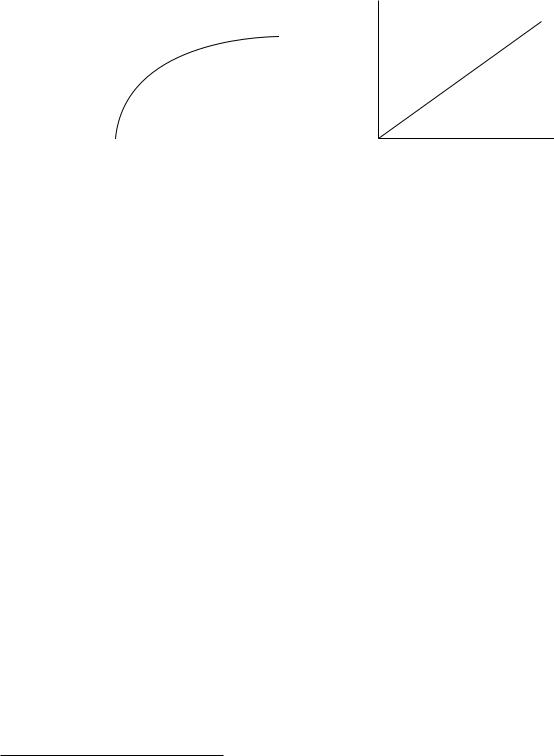
FIGURE 2.1 Production functions. (A) satisfies the Inada conditions in Assumption 2, while (B) does not.
are highly productive and that when capital or labor are sufficiently abundant, their marginal products are close to zero. The condition that F (0, L, A) = 0 for all L and A makes capital an essential input. This aspect of the assumption can be relaxed without any major implications for the results in this book. Figure 2.1 shows the production function F (K, L, A) as a function of K, for given L and A, in two different cases; in panel A the Inada conditions are satisfied, while in panel B they are not.
I refer to Assumptions 1 and 2, which can be thought of as the neoclassical technology assumptions, throughout much of the book. For this reason, they are numbered independently from the equations, theorems, and proposition in this chapter.
2.2 The Solow Model in Discrete Time
I next present the dynamics of economic growth in the discrete-time Solow model.
2.2.1Fundamental Law of Motion of the Solow Model
Recall that K depreciates exponentially at the rate δ, so that the law of motion of the capital stock is given by
K(t + 1) = (1 − δ) K(t) + I (t), |
(2.8) |
where I (t) is investment at time t.
From national income accounting for a closed economy, the total amount of final good in
the economy must be either consumed or invested, thus |
|
Y (t) = C(t) + I (t), |
(2.9) |
where C(t) is consumption.2 Using (2.1), (2.8), and (2.9), any feasible dynamic allocation in this economy must satisfy
K(t + 1) ≤ F (K(t), L(t), A(t)) + (1 − δ)K(t) − C(t)
2. In addition, we can introduce government spending G(t) on the right-hand side of (2.9). Government spending does not play a major role in the Solow growth model, thus its introduction is relegated to Exercise 2.7.
2.2 The Solow Model in Discrete Time |
. |
35 |
for t = 0, 1, . . . . The question is to determine the equilibrium dynamic allocation among the set of feasible dynamic allocations. Here the behavioral rule that households save a constant fraction of their income simplifies the structure of equilibrium considerably (this is a behavioral rule, since it is not derived from the maximization of a well-defined utility function). One implication of this assumption is that any welfare comparisons based on the Solow model have to be taken with a grain of salt, since we do not know what the preferences of the households are.
Since the economy is closed (and there is no government spending), aggregate investment is equal to savings:
S(t) = I (t) = Y (t) − C(t).
The assumption that households save a constant fraction s (0, 1) of their income can be expressed as
S(t) = sY (t), |
(2.10) |
which, in turn, implies that they consume the remaining 1 − s fraction of their income, and thus
C(t) = (1 − s) Y (t). |
(2.11) |
In terms of capital market clearing, (2.10) implies that the supply of capital for time t + 1 resulting from households’ behavior can be expressed as K(t + 1) = (1 − δ)K(t) + S(t) = (1 − δ)K(t) + sY (t). Setting supply and demand equal to each other and using (2.1) and (2.8) yields the fundamental law of motion of the Solow growth model:
K(t + 1) = sF (K(t), L(t), A(t)) + (1 − δ)K(t). |
(2.12) |
This is a nonlinear difference equation. The equilibrium of the Solow growth model is described by (2.12) together with laws of motion for L(t) and A(t).
2.2.2 Definition of Equilibrium
The Solow model is a mixture of an old-style Keynesian model and a modern dynamic macro economic model. Households do not optimize when it comes to their savings or consumption decisions. Instead, their behavior is captured by (2.10) and (2.11). Nevertheless, firms still maximize profits, and factor markets clear. Thus it is useful to start defining equilibria in the way that is customary in modern dynamic macro models.
Definition 2.2 In the basic Solow model for a given sequence of {L(t), A(t)}∞t=0 and an initial capital stock K(0), an equilibrium path is a sequence of capital stocks, output levels, consumption levels, wages, and rental rates {K(t), Y (t), C(t), w(t), R(t)}∞t=0 such that K(t) satisfies (2.12), Y (t) is given by (2.1), C(t) is given by (2.11), and w(t) and R(t) are given by (2.6) and (2.7), respectively.
The most important point to note about Definition 2.2 is that an equilibrium is defined as an entire path of allocations and prices. An economic equilibrium does not refer to a static object; it specifies the entire path of behavior of the economy. Note also that Definition 2.2 incorporates the market clearing conditions, (2.6) and (2.7), into the definition of equilibrium. This practice