Материалы / Курсовые работы 2014 / Материалы для курсовых работ 2014 / K9_NodeActivationMultipleAccess

Distributed Channel Access Scheduling

for Ad Hoc Networks

1 Introduction

In this chapter, we present and analyze protocols for time-division multiple access (TDMA) scheduling in ad hoc networks with omni-directional antennas. These protocols use a neighbor-aware contention resolution (NCR) algorithm to elect deterministically one or multiple winners in a given contention context based on the topology information within two hops. In NCR, the identifiers and the current contention context number are used to derive a randomized priority for each contender in a given contention context. A contention context corresponds to a time slot in time-division multiple access schemes, and the contenders of a given node during a contention context are those nodes one and two hops away from the node. Each contender runs NCR to determine locally its eligibility to access the resource in the contention context by comparing its priority with the priorities of the rest of the contenders.

Based on NCR, the node activation multiple access protocol (NAMA) elects nodes for collision-free broadcast transmissions over a single channel. The link activation multiple access (LAMA), the pair-wise link activation multiple access (PAMA), and the hybrid activation multiple access (HAMA) protocols operate over multiple channels that are orthogonal by codes or frequencies to elect either links or nodes for collision-free unicast transmissions, or a mix of broadcast and unicast transmissions. The throughput and delay characteristics of these protocols are studied by analysis and simulation in multihop wireless networks with randomly-generated topologies. The performance of the new protocols is also compared against a well-known static scheduling algorithm based on complete topology information, and the ideal CSMA and CSMA/CA protocols.

After Section 2 reviewing the prior work on schedules channel access in wireless ad hoc networks, Section 3 presents the the neighbor-aware contention resolution algorithm (NCR) and analyzes the packet delay encountered in a general queuing model under certain contention level. Section 4 describes four scheduling protocols based on NCR, including the packet transmission scheduling based on node activation (NAMA) suitable for broadcast transmission, link activation (LAMA) and pair-wise link activation (PAMA) for unicast packet transmission, and hybrid activation (HAMA) for both unicast and broadcast transmissions. Section 5 derives the channel access probabilities of the four protocols in randomly generated ad hoc networks, and compares the throughput of the protocols with that of the ideal carrier sensing multiple access (CSMA) and carrier sensing multiple access with collision avoidance (CSMA/CA) schemes. Section 6 presents the results of simulations that provide further insights to the performance differences among the four scheduling protocols and the corresponding static scheduling approaches based on a unified multiple access scheduling framework UxDMA [22]. Section 7 summarizes the research and proposes open problems in the area.

1

2 Background Review

There has been considerable work on cellular networks using the time division multiple access (TDMA) for data communication. These multiple access protocols allocate reservation slots to resolve contentions and data information slots to transmit data packets. Examples of this type of approach are D-TDMA (Dynamic TDMA) [12], PRMA (Packet Reservation Multiple Access) [19], RAMA (Resource Auction Multiple Access) [18], and DRMA (Dynamic Reservation Multiple Access) [21]. Despite there are many similarities between the medium access control protocols for cellular and ad hoc wireless networks, ad hoc networks present a distinct multi-hop and distributed scenario in nature, and require special considerations in protocol designs. We provide a brief survey of related time division multiplexing approaches that handles the characteristics of ad hoc networks.

Channel access protocols for ad hoc networks can be non-deterministic or deterministic. The nondeterministic approach started with ALOHA and CSMA [15] and continued with several collision avoidance schemes, of which the IEEE 801.11 series standards for wireless LANs [6] being the most popular examples to date. However, as the network load increases, network throughput drastically degrades in these nondeterministic approaches because the probability of collisions rises, preventing stations from acquiring the channel.

On the other hand, deterministic access schemes set up timetables for individual nodes or links, such that the transmissions from the nodes or over the links are conflict-free in the code, time, frequency or space divisions of the channel. The schedules for conflict-free channel access can be established based on the topology of the network, or it can be topology independent.

Topology-dependent channel access control algorithms can establish transmission schedules by either dynamically exchanging and resolving time slot requests [5] [28], or pre-arrange a time-table for each node based on the network topologies. Setting up a conflict-free channel access time-table is typically treated as nodeor linkcoloring problems on graphs representing the network topologies. The problem of optimally scheduling access to a common channel is one of the classic NP-hard problems in graph theory (k-colorability on nodes or edges) [9] [10] [23]. Polynomial algorithms are known to achieve suboptimal solutions using randomized approaches or heuristics based on such graph attributes as the degree of the nodes.

A unified framework for TDMA/FDMA/CDMA channel assignments, called UxDMA algorithm, was described by Ramanathan [22]. UxDMA summarizes the patterns of many other channel access scheduling algorithms in a single framework. These algorithms are represented by UxDMA with different parameters. The parameters in UxDMA are the constraints put on the graph entities (nodes or links) such that entities related by the constraints are colored differently. Based on the global topology, UxDMA computes the node or edge coloring, which correspond to channel assignments to these nodes or links in the time, frequency or code domain.

A number of topology-transparent scheduling methods have been proposed [4] [13] [16] to provide conflict-free channel access that is independent of the radio connectivity around any given node. The basic idea of the topology-transparent scheduling approach is for a node to transmit in a number of time slots in each time frame. The times when node i transmits in a frame corresponds to a unique code such that, for any given neighbor k of i, node i has at least one transmission slot during which node k and none of k's own neighbors are transmitting. Therefore, within any given time frame, any neighbor of node i can receive at least one packet from node i conflict-free. An enhanced topology-transparent scheduling protocol, TSMA (Time Spread Multiple Access), was proposed by Krishnan and Sterbenz [16] to reliably transmit control messages with acknowledgments. However, TSMA performs worse than CSMA in terms of delay and throughput [16].

In general, the medium access control protocols in ad hoc networks have to combat two problems,

2

namely, “hidden terminal problem” [25] and “exposed terminal problem”. The “exposed terminal problem” is exacerbated in providing reliable broadcast services. The two problems are illustrated in Figure 1.

Figure 1: The hidden terminal and exposed terminal problems.

2.1 Dynamic Reservation TDMA

TDMA schemes based on dynamic reservations constitute a commonly adopted approach that adjusts the time slot assignments according the traffic requirements of individual nodes. The reservation can be made by either in-band signaling or out-band signal, where in-band signals are exchanged in the same channel as data traffic, and out-band signaling uses a separate channel for control information exchanges. However, these two methods are equivalent.

Five-Phase Reservation Protocol (FPRP) was designed to produce TDMA broadcast schedule in mobile ad hoc networks [28].

Figure 2: The Five-Phase Reservation Protocol .

As shown in Figure 2, FPRP uses a similar scheme as D-TDMA in that the time is separated into two alternating activities — a reservation period and multiple information transmission periods. A successful time-slot reservation made during the reservation period lasts for a series of information periods, called Information Frames (IFs). each information frame contains multiple time slots, called Information Slots (ISs), which are assigned to individual nodes according to the result of the reservation. Correspondingly, FPRP sets aside a Reservation Slot (RS) for each Information Slot during the reservation period for nodes to contend using five-phase handshakes for M times, as indicated by 1, 2, 3, 4, 5 in Figure 2. Using multiple five-phase handshakes, an information slot can be allocated with high probability.

The five phases are designated according to senders or receivers. The first phase is called “Reservation Request (RR)”, where senders send out probes to the receivers of the communication. If the RR reaches the receiver successfully, the receiver keeps silent in the second phase to indicate a clear channel to the sender. Otherwise, the receiver replies with a “Collision Report (CR)”. If the sender does not hear anything in the

3

channel during the second phase, it is assured of the clear channel, and sends out “Reservation Confirm (RC)” in the third phase so that all the one-hop neighbors know about the reservation. Then the receiver responds with a “Reservation Acknowledgment (RA)” in the fourth phase, which establishes the connection with the sender. Note that an isolated node may get into phase three without any channel response, and only phase four confirms the existence of the receiver. In phase five, called “Packing and Elimination (P/E)”, the neighbors of the receivers send “Packing Packet” to notify their one-hop neighbors that less nodes will compete in the next contention phases. In phase five, senders may also probabilistically send “Elimination Packet” in order to break the tie where two senders are adjacent to each other.

Because of the relative simple meaning of each phase, the handshake packets can be made small enough to indicate the channel busy state, and the five-phase reservation cycle becomes compact.

FPRP resembles IEEE 802.11 DCF [20] in collision avoidance and HiperLAN [8] in sender deadlock elimination. The only difference is that FPRP is a synchronous protocol, requiring tight timing between phases and short propagation delay between nodes, which are stringent in mobile ad hoc networks. In addition to its complexity, the fixed numbers of information frames and reservation cycles in each reservation slot are not suitable in mobile and ad hoc environments where the density, and topology of the network change frequently. Although FPRP successfully avoids the hidden terminal problem, it still suffers from the “exposed terminal problem” with certain “deadlock” probability as shown in the fifth phase in FPRP. Therefore, FPRP can only provide reliable broadcast schedules with high probability.

Other approaches in the same reservation-based vein differ in the handshaking procedures and the arrangement of reservation phases with regard to the data transmission phases, such as [5] and [24].

2.2 Graph Theoretic Approaches

Besides the various contention based resource reservation protocols, the channel access problem is often reduced to graph coloring problems, where the edge-coloring and node-coloring solutions are directly applied to the link-activation and node-activation schemes of the channel access problems in ad hoc networks.

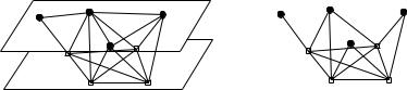
In [9], Ephremides and Truong proved that the optimal broadcast scheduling problem (BSP) in ad hoc networks is NP-complete by showing that the well-known NP-complete problem of finding the maximum independent set (MIS) in a graph reduces to the broadcast scheduling problem. We briefly describe the reduction steps.

The basic approach in reducing the maximum independent set of a graph is to add a vertex for each edge in the graph, and connect the vertex with the end-points of the edge. In addition, the newly added vertexes are fully connected.

G

1

G’

2

Figure 3: The Reduction of Maximum Independent Set to Broadcast Schedule.

For instance in Figure 3 (a), the original graph G is place in plane 1, and the added vertexes are in plane 2. When the original edges are removed, which gives a reduced graph G0 in Figure 3 (b). Because a broadcast schedule requires the set of broadcasting nodes be separated by at least two hops to avoid hidden terminal problem, it is easy to see that the maximum broadcast set in G0 consists of vertexes only from the original graph G. Otherwise there can be only one broadcast vertex if it is selected from plane 2. Then,

4

finding the maximum broadcast set in G0 is identical to finding the maximum independent set of graph G, vice versa.

A distributed implementation of finding the maximal-throughput broadcast schedule was provided in [9], which starts from a simple and inefficient time slot assignment and iteratively assigns more spatially reusable time slots. The drawback of the approach is that the convergence of the algorithm is proportional to the diameter of the network topology. Because the distributed protocol is sensitive to topological change, a topological change may required computing the broadcast schedule from scratch.

Channel assignment problems in the time, frequency and code domains are studied in other works as well. Ramanathan explored a set of eleven atomic “constraints” that characterize the assignment problems within and across these domains, and introduced a unified framework, called UxDMA (Unified T/D/C Division Multiple Access), for the study of assignment problems using graph coloring algorithms. Most assignment problems can be represented as various combinations of these atomic constraints. We describe UxDMA as follows.

In UxDMA, a wireless network is represented as a directed graph G = (V; A), where V is a set of vertexes denoting the nodes in the network, and A is a set of directed edges between vertexes representing wireless links in the network. A directional edge (i; j) 2 A means vertex v can receive packets from vertex u. Communication constraints over the shared wireless media in the frequency, time and code division domains are shown in Figure 4, which illustrates the eleven atomic relations between vertexes and directional edges. The solid dots are transmitters, and the circles are receivers. Wide lines indicate that the lines are activated, and thin lines are interferences.

Figure 4: Constraints used by UxDMA for channel access scheduling.

A constraint is represented using syntax Xzy , where X indicates whether the constrained entities are vertexes or edges, y indicates separation distance between the constrained entities, and z indicates the transmission or reception relation between the constrained entities. For instances, constraints Vtt1, Err0 and Etr1 forbids hidden terminal problem in the channel access schedules, while Vtr1 and Ett1 forbids exposed terminal problem in the channel access schedules, as shown in Figure 1.

Assignment problems are characterized by a set of constraints. For instance, C = fVtr0 ; Vtt1; Vtr1 g is a constraint set for broadcast scheduling. An assignment problem specified by a constraint set requires an assignment that eliminates all the possible scenarios in the constraint set. For instance, a broadcast schedule under constraint set C = fVtr0 ; Vtt1; Vtr1 g forbids that two vertexes can have the same color if they are either

adjacent (Vtr0 , Vtr1 ) or have a common neighbor (Vtt1).

Given the constraint set of a channel access scheduling problem, the coloring of the graph becomes an orderly procedure on the vertexes or edges based on certain heuristics, such as “maximum-degree vertex

5

first” approach. Each step walks through uncolored vertexes in the ordered list of vertexes, and the minimum unused color is found and assigned to a vertex or an edge, subject to the constraint set with regard to the already colored vertexes or edges. Such steps repeat until all the entities in the graph are colored. As we can see, the complexity of the UxDMA for any channel access scheduling problem is polynomial based on the heuristics.

UxDMA can represent a large class of channel access problems, and provides a theoretic bound for such problems. However, just like other approaches that studies the channel access problems from a centralized point of view, the scalability and adaptiveness of such algorithms in mobile ad hoc network are the main issues.

2.3 Topology-Transparent Scheduling

Schedules based on time division multiplexing (TDM) depends critically on the actual network topology, so in a mobile environment, due to nodal mobility and potentially rapid change of topology, TDM schemes may require prohibitive overhead associated with constant updating of schedules.

Several approaches based on the topology-transparent scheduling schemes that are based on different theories have been proposed [3] [4] [13] [14] to reduce the overheads incurred from the conflict-free schedule maintenance. However, they require that the maximum number of nodes and the maximum degree of nodes in the network is known beforehand to guarantee successful transmission of each data frame to all one-hop neighbors.

The Time-Spread Multiple Access (TSMA) proposed by Chlamtac et al. [3] [4], and further refined by Ju et al. [13] uses polynomials over Galois fields to produce appropriate TSMA codes, and assigns them to the network nodes. In addition, Ju and Li proposed another topology-transparent channel access scheduling approach based on Latin Squares [7] for ad hoc networks with multiple channels [14].

A Latin square of order n is defined as an n n matrix composed of n symbols f1; 2; : : : ; ng such that symbols in each row and column are distinct. Two Latin squares A = (ai;j ) and B = (bi;j ) are said to be orthogonal if the n2 ordered pairs (ai;j ; bi;j ) are all different. For examples, the following two square matrices A and B using symbols f1; 2; 3; 4g are both Latin squares, and mutually orthogonal. Generally, latex squares A(1) , A(2) , : : :, A(r) form an orthogonal family if every pair of them is orthogonal.

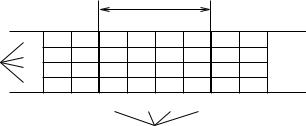
The TDMA scheduling algorithm in [14] maps a p p Latin square onto an M p time division multiple channels, where the number of channels is M , and the number of time slots in each frame is p. Then it assigns a unique symbol from the Latin square to each node, and the positions of the symbol in the Latin square determines the time slots assigned to the node.

For example, in Figure 5, a network is given four channels, and each frame contains four time slots. The assignments of time slots are given in the figure according to the symbols 1, 2, 3, 4 in the Latin square A given above. Therefore, if a node is assigned symbol 2, it can access the first channel in time slot 2, the second channel in time slot 1, the third channel in time slot 4, and the fourth channel in time slot 3.

In addition, it is assumed that each node is equipped with p receivers for all the channels, and one transmitter to send data frames in the assigned time slots. Each data frame is transmitted for p times in each time frame.

However, the available symbols would have been scarce if only p symbols are available to networks with more than p nodes. This is where the orthogonal Latin matrices come into the solution in [14] by assigning the same symbol from different orthogonal Latin matrices to nodes. This is explained as follows.

6

Time Slots

Figure 5: Multi-Channel TDMA Time Frame Structure.

From the definition of orthogonal matrix, we know that any pair of order symbol (a; b) appears at most once in all positions of two orthogonal matrices. Therefore, the symbol/time slot assignments to two nodes conflict in one position at most. Given that a data frame is transmitted multiple times in multiple channels, the successful transmission chances between two nodes are guaranteed. By requiring the minimum order of the orthogonal matrices, which is a function of the nodal degree, the number of collisions at a node from other neighbors with different symbol assignments is kept below p. Consequently, every data frame from a node can be successfully received by its neighbors in one of the p transmissions. Given an orthogonal Latin matrix family of r members, a total of p r symbols can be assigned in a network.

Overall, the topology-transparent TDMA scheme based on Galois Field needs only a single channel and multiple frames for each transmission session, while the scheme based on Latin square specifies a multiple channel TDMA scheduling protocol. It remains to be proved that these approaches based on Galois field and Latin square are based on the same theory because of their many similarities.

3 Neighbor-Aware Contention Resolution

3.1 Specification

The neighbor-aware contention resolution (NCR) solves a special election problem where an entity to locally decide its leadership among a known set of contenders in any given contention context. We assume that the knowledge of the contenders for each entity is acquired by some means. For example, in the ad hoc networks of our interest, the contenders of each node are the neighbors within two hops, which can be obtained by each node periodically broadcasting the identifiers of its one-hop neighbors [1]. Furthermore, NCR requires that each contention context be identifiable, such as the time slot number in networks based on a time-division multiple access scheme.

We denote the set of contenders of an entity i as Mi, and the contention context as t. To decide the leadership of an entity without incurring communication overhead among the contenders, we assign each entity a priority that depends on the identifier of the entity and the current contention context. Eq. (1) provides a formula to derive the priority, denoted by i.prio, for entity i in contention context t.

where the function Hash( ) is a fast message digest generator that returns a random integer in a predefined range, and the sign ` ' is designated to carry out the concatenation operation on its two operands. Note that, although the Hash( ) function can generate the same number on different inputs, each priority number is unique because the priority is appended with identifier of the entity.

7

NCR(i, t) f

/* Initialize. */

1for (k 2 Mi [ fig)

2k.prio = Hash(k t) k;

/* Resolve leadership. */

3if (8k 2 Mi ; i:prio > k:prio)

4i is the leader;

g /* End of NCR. */

Figure 6: NCR Specification.

Figure 6 shows the NCR algorithm. Basically, NCR generates a permutation of the contending members, the order of which is decided by the priorities of all participants. Since the priority is a pseudo-random number generated from the contention context that changes from time to time, the permutation also becomes random such that each entity has certain probability to be elected in each contention context, which is inversely proportional to the contention level as shown in Eq. 2.

Conflicts are avoided Because it is assumed that contenders have mutual knowledge and t is synchronized, the order of contenders based on the priority numbers is consistent at every participant.

3.2 Dynamic Resource Allocation

The description of NCR provided so far evenly divides the shared resource among the contenders. In practice, the demands from different entities may vary, which requires allocating different portion of the shared resource. There are several approaches for allocating variable portion of the resource according to individual demands. In any approach, an entity, say i, needs to specify its demand by an integer value chosen from a given integer set, denoted by pi. Because the demands need to be propagated to the contenders before the contention resolution process, the integer set should be small and allow enough granularity to accommodate the demand variations while avoiding the excess control overhead caused by the demand fluctuations.

Suppose the integer set is f0; 1; ; P g, the following three approaches provide resource allocation schemes, differing in the portion of the resource allocated on a given integer value. If the resource demand is 0, the entity has no access to the shared resource.

3.2.1Pseudo identities

An entity assumes p pseudo identities, each defined by the concatenation of the entity identifier and a number from 1 to p. For instance, entity i with resource demand pi is assigned with the following pseudo identities: i 1, i 2, , i pi. Each identity works for the entity as a contender to the shared resource. Figure 7 specifies NCR with pseudo identities (NCR-PI) for resolving contentions among contenders with different resource demands.

The portion of the resource available to an entity i in NCR-PI according to its resource demand is as

8

NCR-PI(i, t) f

/* Initialize each entity k with demand pk . */

1for (k 2 Mi [ fig and 1 l pk )

2(k l).prio = Hash(k l t) k l;

/* Resolve leadership. */

3if (9k; l : k 2 Mi ; 1 l pk and

48m : 1 m pi ; (k l):prio > (i m):prio)

5i is not the leader;

6else

7i is the leader;

g /* End of NCR-PI. */

Figure 7: NCR-PI Specification.

3.2.2Root operation

Assuming enough computing power for floating point operations at each node, we can use the root operator to achieve the same proportional allocation of the resource among the contenders as in NCR-PI.

Given that the upper bound of function Hash in Eq. (1) is M , substituting line 2 in Figure 6 with the following formula generates a new algorithm which provides the same resource allocation characteristic as shown in Eq. (3).

3.2.3Multiplication

Simpler operations, such as multiplication in the priority computation, can provide non-linear resource allocation according to the resource demands. Substituting line 2 in Figure 6, Eq. (5) offers another way of computing the priorities for entities.

According to Eq. (5), the priorities corresponding to different demands are mapped onto different ranges, and entities with smaller demand values are less competitive against those with larger demand values in the contentions, thus creating greater difference in resource allocations than the linear allocation schemes provided by Eq. (3) and Eq. (4). For example, among a group of entities, a, b and c, suppose pa = 1,

For simplicity, the rest of this chapter addresses NCR without dynamic resource allocation.

3.3 Performance

3.3.1System delay

We assume NCR as an access mechanism to a shared resource at a server (an entity), and analyze the average delay experienced by each client in the system according to the M/G/1 queuing model, where clients arrive at the server according to a Poisson process with rate and are served according to the first-come-first- serve (FIFO) discipline. Specifically, we consider the time-division scheme in which the server computes

9

the access schedules by the time-slot boundaries, and the contention context is the time slot. Therefore, the queuing system with NCR as the access mechanism is an M/G/1 queuing system with server vacations, where the server takes a fixed vacation of one time slot when there is no client in the queue at the beginning of each time slot.

The system delay of a client using NCR scheduling algorithm can be easily derive from the extended Pollaczek-Kinchin formula, which computes the service waiting time in an M/G/1 queuing system with server vacations [2]

where X is the service time, and V is the vacation period of the server.

According to the NCR algorithm, the service time X of a head-of-line client is a discrete random variable, governed by a geometric distribution with parameter q, where q is the probability of the server accessing the shared resource in a time slot, as given by Eq. (2). Therefore, the probability distribution function of

service time X is

P fX = kg = (1 q)k 1q ;

where k 1. Therefore, the mean and second moments of random variable X are:

Because V is a fixed parameter, it is obvious that V = V 2 = 1. Therefore, the average waiting period in the

Adding the average service time to the queuing delay, we get the overall delay in the system:

Average Packet Delays in the System

Figure 8: Average system delay of packets.

The probabilities of the server winning a contention context are different, and so are the delays of clients going through the server. Figure 8 shows the relation between the arrival rate and the system delay of clients in the queuing system, given different resource access probabilities. To keep the queuing system in a steady state, it is necessary that < q as implied by Eq. (6).

10