1 / 20701

lines is not zero, voltage harmonics appear. Particularly important is the measurement and analysis of possible adverse effects of harmonics on the equipment connected to the network. Power quality analyzers that measure the harmonic content in the supply voltage are too expensive to apply at each node where the renewable source is connected to the network.

Fast Backup Switch-on

Fig. 1. A structure of protection, monitoring and control system integrating distributed renewable energy sources and energy containers

The solution to the problem of mass scale power quality monitoring and control is to equip conventional protection relays with power quality analysis functions, Figure 2. The natural nodes to place the combined devices are at the output of the inverters marked in Figure 2 by red color. The tremendous advance in the DSP microprocessor technology enables to implement the power quality analysis software, particularly harmonics and interharmonics level determination, at a very small additional cost for the end user. The advanced signal processing algorithms like signal resampling in the digital domain are the key to achieving design objectives. To keep the cost of the developed protection relay low, the developed algorithms should put minimal requirements on hardware.

www.intechopen.com

parameters like RMS, which are then used by protection algorithms. In this respect they are similar to stand alone power quality analysers that also carry out the calculations of signal parameters from sample sequences. The availability of fast and high resolution analogue to digital converters enables cost effective signal front end design suited equally well for protection relay and power quality analyser.

Fig. 3. Block diagram of combined protection relay and power quality analyser

The architecture of combined protection relay and power quality analyser has been shown in Figure 3. The architectures of power quality analyzer and protection relay are very similar. They differ only in the transient voltage surge measurement module, which has been marked by a different colour in Figure 3. While the basic signal parameterization software implemented in both devices uses Fourier techniques for spectrum determination, the protection relays contain additionally the protection algorithms software and power quality analyzers contain more elaborate spectrum analysis and statistical software. Power quality analyzers also have wider input bandwidth to measure accurately harmonic and interharmonic content of the signal up to 2 kHz. To merge protection relay and power quality analyser in a single device in a cost effective way it is necessary to employ advanced signal processing techniques like oversampling and changing the effective sampling rate in digital domain.

www.intechopen.com

2.1 Harmonic and interharmonic content determination 2.1.1 Introduction

The international standards concerning power quality analysis (EN 50160, EN 61000-4- 7:2002, EN 61000-4-30:2003) define precisely which parameters of line voltage and current signals are to be measured and the preferred methods of measurement in order to determine power quality. In compliance with these requirements, for harmonic content determination, power quality analyzers employ sampling procedures with sampling frequency precisely synchronized to the exact multiple of line frequency. This is necessary for correct spectrum determination as is known from Fourier theory (Oppenheim & Schafer, 1998). If the sampling frequency is not equal to the exact multiple of line frequency, the spectral components present in the signal are computed with error and moreover false components appear in the spectrum.

Efficient computation of signal spectrum with the use of FFT transform demands that the number of samples in the measurement interval be equal to the power of two. With sampling frequency synchronized to the multiple of line frequency, it is impossible to satisfy this requirement both in one line period measurement interval – when the measurement results are used for protection functions, and ten line periods measurement interval when interharmonic content is determined. This is the reason why some power quality analyzers available on the market offer interharmonic content measurement over 8 or 16 line periods interval. Another disadvantage of synchronizing sampling frequency to the line signal frequency is the inability to associate with each recorded signal waveform sample a precise moment in time. When the power quality meter is playing also the role of disturbance recorder, the determination of a precise time of an event is very difficult in such case. A better method to achieve the number of samples equal to the power of two both in one and ten line periods, with varying line frequency, is to use constant sampling frequency and employ digital multirate signal processing techniques.

As the digital multirate signal processing involves a change in the sample rate, the sampling frequency can be chosen with the aim of simplifying the antialiasing filters that precede the analog to digital converter. According to the EN 61000-4-7:2002 standard, the signal bandwidth that has to be accurately reproduced for power quality determination is 2 kHz. The complexity of the low-pass filter preceding the A/D converter depends significantly on the distance between the highest harmonic in the signal that has to be passed with negligible attenuation (in this case the 40-th harmonic) and the frequency equal to the half of the sampling frequency. When the sampling frequency around 16 kHz is chosen, a simple 3- pole RC active filter filters can be used.

2.1.2 Multirate digital signal processing in protection relay

In multirate digital signal processing (Oppenheim & Schafer, 1998) it is possible to change the sampling rate by a rational factor N/M using entirely digital methods. The input signal sampled with constant frequency fs is first interpolated by a factor of N and then decimated by a factor of M – both these processes are called collectively resampling. The output sequence consists of samples representing the input signal sampled at an effective frequency fseff , where

The first thing that has to be determined is how many samples are needed to calculate the spectral components of the signal. For protection purposes, the knowledge of harmonics up

www.intechopen.com

to 11th used to be enough in the past. The increasing use of nonlinear loads (and competition) has led leading manufacturers of protection relays to develop devices with the ability to determine the signal spectrum up to 40 or even 50-th harmonic. Thus, taking into account that the number of samples, for computational reasons, must equal the power of two, 128 samples per period are needed (Oppenheim & Schafer, 1998). The ideal sampling frequency is then fsid = fline · 128 Hz (= 6400 Hz at 50 Hz line frequency). For power quality analysis, the EN 61000-4-7 standard demands that the measurement interval should equal ten line periods and the harmonics up to 40th (equivalently interharmonics up to 400th) have to be calculated. This gives 1024 as the minimum number of samples over ten line periods meeting the condition of being equal to the power of two. The ideal sampling frequency fsid for interharmonic content determination should be equal to ((fline)/10) · 1024 Hz which is 5120 Hz at fline = 50 Hz. Knowing the needed effective sampling frequency and the actual sampling frequency fs – which for the rest of the chapter is assumed to be equal to 16 kHz, the equation (1) can be used to determine interpolation and decimation N, M values. Tables 1 and 2 gather the values of N and M (without common factors) computed from (1) for a range of line frequencies.

Table 2, cont.

For some line frequencies the values of N and M computed from (1) are very large, e.g. for fline = 49.991 Hz, N = 49991 and M = 125000. The computational complexity of the resampling procedure depends on how large the values of N and M are.

www.intechopen.com

The interpolation process consists in inserting a N-1 number of zero samples between each original signal sample pair. The resulting sample train corresponds to a signal with the bandwidth compressed with N ratio and multiplied on a frequency scale N times (Oppenheim & Schafer, 1998). To recover the original shape of the signal, the samples have to be passed through a low pass filter with the bandwidth equal to the B/N bandwidth of the signal prior to interpolation. In time domain the filter interpolates the zero samples that have been inserted between the original signal samples.

XHL(ejω)

Fig. 4. The effect of interpolation and decimation on signal spectrum

The decimation process consists in deleting M-1 samples from each consecutive group of M samples. The resulting sample train corresponds to a signal prior to the decimation but with the bandwidth expanded by a factor of M. To prevent the effect of aliasing, the sample sequence to be decimated has to be passed through a low pass filter with the bandwidth equal to 2π/M in normalized frequency. The operation of interpolation and decimation on the bandwidth of the signal has been shown in Figure 4 for N = 2 and M = 3. In this figure X(ejω) is the spectrum of the original signal, XL(ejω) is the spectrum of the original signal with zero samples inserted and XLM(ejω) the spectrum of the original signal with zero samples inserted and then decimated with the M ratio. As can be seen in Figure 4 c) there is a frequency aliasing. If the signal after interpolation is passed through a low pass filter with suitable frequency characteristic H(ejω) the effect of frequency aliasing is avoided as shown in Figure 4 d).

To preserve as much of the bandwidth of the original signal as possible, the low pass filter used in the resampling process has to have a steep transition between a pass and stop bands. The complexity of the filter depends heavily on the magnitude of the greater of the values of N and M. This is one of the many reasons why the values of N and M should be

www.intechopen.com

chosen as low as possible but at the same time the feff computed from (1) should be as close as is necessary to the ideal sampling frequency fsid.

The accuracy with which feff is to approximate fsid could be determined from simulating how different values of N and M affect the accuracy of spectrum determination. However some clues about the values of N and M can be obtained from EN 61000-4-7 standard. In chapter 4.4.1 it states that the time interval between the rising edge of the first sample in the measurement interval (200 ms in 50 Hz systems) and the rising edge of the first sample in the next measurement interval should equal 10 line periods with relative accuracy not worse than 0.03%. Therefore, for each line frequency, the values of N and M should be chosen so as the relative difference Eeff between the ideal sampling frequency fsid, and the effective sampling frequency feff meets the following condition

The frequency characteristic of the low pass filter used in the resampling procedure depends on the values of N and M. If a different filter is used for each N, M pair it places a heavy burden on limited resources of DSP processor system in a protection relay. A solution to this problem is to fix the value of N and choose M according to the following formula

where L is the number of periods used in the spectrum determination and SN is the number of the samples in L periods (128 samples per one period for protection functions, 1024 samples per 10 periods for power quality analysis). The Round(x) function gives the integer closest to x. The low pass filter is then designed with the bandwidth equal to 2π/Mmin where Mmin is the value of M computed from (2) for highest line frequency fline.

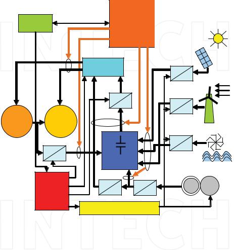
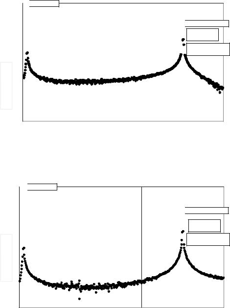
For power quality analysis when the interharmonics content has to be determined, N=600, the minimum value of M is 1630 at fline = 57.5 Hz, the maximum value of M is 2206 at fline = 42.5 Hz. The maximum absolute value of Eeff is equal to 0.03% and the effective sampling frequency is within the range recommended by EN 61000-4-7 standard. As the error of spectrum determination increases with increasing Eeff it is sufficient to carry out the analysis of the accuracy of spectrum determination for line frequency, for which the Eeff is largest. The obtained accuracy should then be compared with the accuracy of spectrum determination when the sampling frequency is synchronized to the multiple of the same line frequency with the error of 0.03%. For the analysis a signal composed of the fundamental component, 399 interharmonic with 0.1 amplitude relative to the fundamental, 400 interharmonic with 0.05 amplitude relative to the fundamental and 401 interharmonic with 0.02 amplitude relative to the fundamental should be selected. This is the worst case signal because on the one hand the error is greatest at the upper limit of the frequency range, and on the other hand when close interharmonics are present, there is leakeage from the strongest interharmonic to the others. Figure 5 shows the spectrum of the test signal determined when the synchronization technique is used and Figure 6 shows the spectrum when the digital resampling technique is used. In both cases the resulting sample rate is identical.

www.intechopen.com

The two spectra are almost identical and they both give the same error in the interharmonic level determination. The level of 399th interharmonic is very close to the true value. However the level of 40th harmonic is almost three times higher than the true value and the level of 401st interharmonic is almost four times higher than the true value. The observed effect can be explained by leakage of the spectrum from 399th interharmonic of relatively large level to neighbouring interharmonics (Bollen & Gu 2006). The detailed analysis carried out for the whole range of line frequency and various signal composition shows that if the error between the ideal sample rate and actual sample rate at the input of Fourier spectrum computing procedure is the same, both methods give equally accurate results.

For the protection functions the needed frequency resolution is ten times lower than for interharmonic levels determination. It suggests, that the values of N and M can be chosen such that the maximum value of Eeff < 0.3%. With N=80, the minimum value of M equal to 174 at fline = 57.5 Hz, and the maximum value of M equal to 235 at fline = 42.5 Hz, the maximum absolute value of Eeff is equal to 0.284%. The detailed analysis shows that harmonics are determined with the accuracy which is better than 1%.

3. New input circuits used for parameters determination of line current and voltage signals

The measurement of line voltage and current signals for power quality analysis demands much higher accuracy than is needed for protection purposes. Traditional voltage and current transducers used in primary circuits of power stations cannot meet the requirements of increased accuracy and wide measurement bandwidth. New types of voltage and current transducers are needed with frequency measurement range equal to at least the 40-th harmonic of fundamental frequency, high dynamic range and very good linearity. For current measurements Rogowski coils may be used. They have been used for many years in applications requiring measurements of large current in wide frequency bandwidth. The traditional technologies used for making such coils were characterized by large man labour. Research work has been carried out at many laboratories to develop innovative technologies for Rogowski coil manufacture. These technologies are based on multilayer PCB.

3.1 Principle of PCB Rogowski coil construction

The principle of Rogowski coil operation is well known (http://www.axilane.com/PDF_Files/Rocoil_Pr7o.pdf). The basic design consists in winding a number of turns of a wire on a non-magnetic core, Figure 7.

The role of the core is only to support mechanically the windings. The voltage V(t) induced at the terminations is expressed by the following equation

where µ0 is the magnetic permeability of the vacuum, n is the number of turns, A is the area of the single turn (referring to Figure 7, A=π·r2) and I is the current flowing in the conductor coming through the coil.

www.intechopen.com