7. Forms of representation of a line in the space.

There are different ways of representation of a line in the space in some Cartesian system of coordinates .

1. An equation of a line in parametric form. Let a point with the radius-vector lies on a line in the space having non-zero directing vectorand passing through a point. Then collinearity of vectorsandimplies that an equation of line in the space must have the form:.

2. An equation of a line in canonic form. If we exclude parameter from the scalar record of the equation:then we obtain so-calledcanonic equation of line:

.

3. An equation of a line passing through two non-coinciding points and .

Since directing vector of the line is collinear to vector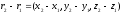, an equation of line in vector form can be represented asor.

Excluding parameter , we obtain an equation in the coordinate form:

only if .

4. An equation of a line in the first vector form. A line in the space can be given as a line of intersection of two planes andwhereandare non-collinear, normal vectors of these planes, andandare some numbers.

If it is known a point which is passed through by a given line then the radius-vector of any point of this line satisfies to the following system of equations:or in the coordinate form:.

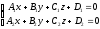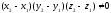
5. An equation of a line in the second vector form. A line in the space can be given by means of the condition of collinearity of vectors and, i.e.orwhere.

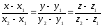
In an orthonormal system of coordinates this equation of line in the space is:

or .

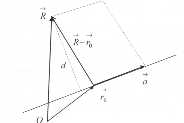
At last, the distance between some point with the radius-vectorand a linein the space can be found by using thatis the area of parallelogram constructed on the pair of vectors is equal to the module of their vector product.

.

8. Curves of the second order in plane: theorem on canonic forms (case B = 0). Canonic system.

Let an orthonormal system of coordinates and some curvebe given on a plane.

A curve is called analgebraic curve of the second order if its equation in a given system of coordinates has the form:

where numbers andare not equal to zero simultaneously (), andandare the coordinates of the radius-vector of a point lying in the curve.

Introduce the following notation: .

Theorem 1. For every curve of the second order there exists an orthonormal system of coordinates in which an equation of this curve has (for) one of the following nine (calledcanonic) forms:

Type of curve
Empty sets
Points
Coinciding lines
Non-coinciding lines
Curves	Ellipse	Hyperbola	Parabola

Remark 1. Curves of the second order for which are related to anelliptic type, curves with – to ahyperbolic type, and curves with – to aparabolic type.

Remark 2. In order to find the canonic system of coordinates (i.e. the system of coordinates in which an equation has a canonic form) we write each of transition formulas, substitute them each other and obtain a final expression of the original coordinates through canonic ones:

The coefficients of these formulas give the coordinates of the origin of canonic system of coordinates and its basis vectorsregarding to the original system.