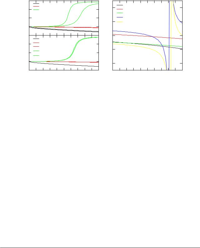
Figure 3.3: The phase shifts (E) and the corresponding logarithmic derivatives D (E) of Fe in the ordered compound FeCo.

3.3Plotting of wave functions

The valence band and core level wave functions used by the SPRKKR package may be ploted using kkrgen. The specific part of the input file DATASET.inp supplies the following parameters:

section TASK

24

section ENERGY

The energy dependent spin-orbit-splitting parameters l(E) are written to files, that can be used directly by xmgrace.

Files used:

25

Example

The input file to plot the d-like wave functions of Fe in FeCo should look like this:

###############################################################################

# SPR-KKR input file FeCo_WFPLOT.inp

# created by xband on Sat Jan 22 17:45:12 CET 2005

###############################################################################

#STATE=CORE CL=2p mj=+1/2

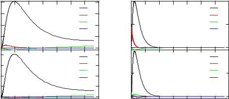
The run of kkrgen creates the wave function files to be viewed directly via xmgrace. A run with the input file shown above and a second one for the 2p-core levels leads to the results shown in Fig. 3.4.

Figure 3.4: The valence band d-electron (left) and 2p-core state (right) wave function for Fe in FeCo. The core wave functions have been created in a second run of kkrgen.

26

3.4Spin-orbit parameter

The spin-orbit-splitting parameter l(E) depends on the energy E and can be calculated l- resolved using kkrgen with an input and potential file supplied. The specific part of the input file DATASET.inp supplyies the following parameters:

section TASK

VAR / SWITCH default description

The energy dependent spin-orbit-splitting parameters l(E) are written to files, that can be used directly by xmgrace.

Files used:

27

Example

To calculate the spin-orbit-splitting parameter l(E) for the ordered compound FeCo the input file created by xband should look like this:

###############################################################################

# SPR-KKR input file FeCo_SOCPAR.inp

# created by xband on Mon Jan 17 22:05:32 CET 2005

###############################################################################

CONTROL DATASET = FeCo

ADSI = SOCPAR

POTFIL = FeCo.pot

PRINT = 0

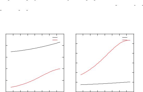
The file FeCo.pot has to contain the (usually converged) potential created by kkrscf. Running kkrgen the energy-dependent spin-orbit-splitting parameter l(E) will be written to the files FeCo SOCPAR soc Fe.agr and FeCo SOCPAR soc Co.agr. In addition an effective energy-dependent exchange splitting Exc is written to the files FeCo SOCPAR exc Fe.agr and FeCo SOCPAR exc Co.agr. All these files can be viewed directly using xmgrace, i.e. there is no need for post-processing. As an example the spin-orbit-splitting parameter of Fe

in FeCo is shown in Fig. 3.5.

Figure 3.5: The energy dependent spin-orbit-splitting and exchange splitting parametersl(E) and Exc, repectively, for p- and d-electrons of Fe in FeCo.

28

3.5 Dispersion relation ~ E(k)

coordinates with * = 1; :::;NKDIR

The dispersion relation ~ is calculated for an energy range fixed by the variables

E(k) EMIN and EMAX with the accuracy determined by the energy step (EMAX-EMIN)/(NE-1). There

are two ways to specify the corresponding path in ~-space: k

select a predefined path by using the variable KPATH. See the list above for the available settings.

specify the number NKDIR of segments of a user defined path and give for all segments

the first and last ~-vectors. k

kkrgen determines the dispersion relation ~ from the number of positive eigen

E(k) N(E)

values of the KKR-matrix. For are given ~ is calculated for every energy value of the k N(E)

mesh specified by NE, EMIN, and EMAX. An energy eigen value is indicated by a change in N(E) for increasing E. kkrgen uses the constant-E mode to calculate the dispersion relation. This may lead to rather long execution times.

kkrgen writes the result to a file DATASET.bnd. Use plot to convert the data to a xmgrace file.

Files used:

29

on the path in ~-space. Use plot to obtain the corre- k

sponding xmgrace file.

30

Example

To calculate the density of states for the ordered compound FeCo the input file created by xband should look like this:

###############################################################################

###############################################################################

The file FeCo.pot has to contain the (usually converged) potential created by kkrscf. Running kkrgen the density of states data will be written to the file FeCo DOS.dos. The content of the file can be viewed using plot via xband. For the present example one gets the three files FeCo DOS.dos.agr, FeCo DOS.dos Co.agr, and FeCo DOS.dos Fe.agr, that give the total and partial DOS and that can be viewed by invoking xmgrace. As an example the partial DOS of Fe is shown in Fig. 3.9. Note that the energy range is given in the input file in

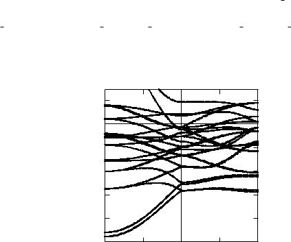
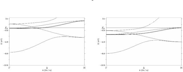
Figure 3.6: The dispersion relation ~ of FeCo for the wave vector ~ along the path

E(k) k

X M.

units of Ry with respect to the muffin-tin zero. For the display of the DOS the energy range is converted to eV with respect to the Fermi energy, i.e. E = 0 corresponds to E = EF .

31

32 CHAPTER 3. ELECTRONIC STRUCTURE CALCULATIONS

The Bloch spectral function AB(E; k) can be seen as a k-resolved DOS function [11]. For an

ordered system it is a -like function, that carries the same information as the dispersion

represent the electronic band structure. The Bloch spectral function ~ is obtained by

AB(E; k)

running kkrgen with appropriate potential and input files. The specific part of the input file DATASET.inp supplyies the following parameters:

in ~-space k

32

Example

To calculate the spin-resolved Bloch spectral function (BSF) for bcc-Fe the input file created by xband should look like this:

###############################################################################

###############################################################################

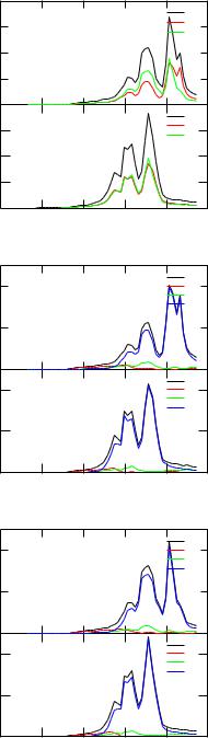
The file Fe.pot has to contain the (usually converged) potential created by kkrscf. Running kkrgen the BSF will be written to the file Fe BLOCHSF.bsf, which then can be visualised using plot from within xband.

Figure 3.7: Spin-up (left) and spin-down (right) BSF for bcc-Fe.

Furthermore, one can also calculate different cuts through Fermi surfaces. For this, the xband created inputfile should look like this:

34

###############################################################################

###############################################################################

Note, that the parameters EMIN and EMAX must be set to the Fermi energy which is obtained from the converged potential file. created by kkrscf. Running kkrgen the data will be written to the file Fe BLOCHSF.bsf, which then can be visualised using plot from within xband.

Figure 3.8: Cut by -H -H-plane through the Fermi surface of bcc-Fe. Spin-up and spindown BSF are shown on the left and right panels, respectively.

35

3.7Density of States n(E)

To calculate the angular momentum, spin and component resolved density of states (DOS) n(E) run kkrgen supplying an input and potential file. In addition the -resolved DOS and the spin and orbital polarizations, P spin= dh zi=dE and P orb= dhlzi=dE, can be obtained.

The specific part of the input file DATASET.inp supplyies the following parameters:

See Fig. 3.1 for a graphical representation of the various paths in the complex energy plane.

36

kkrgen writes the following information to standard output:

-------------------------------------------------------------------------------

This block is printed for every energy and component IT and gives the DOS, spin-polariza- tion P spin= dh zi=dE, orbital polarization P orb= dhlzi=dE, and valence band hyperfine field in their integrated (INT(DE)) and differential form. The full values (crystal) as well as their back scattering parts are given separately. These are obtained from Eq. (1.11) by ig-

noring the second irregular part and replacing nn00 (E) by nn00 (E) tn 0 (E). For IPRINT 1 a decomposition according to the magnetic quantum number is given in addition.

kkrgen stores the calculated DOS in the file DATASET.dos. Use plot to convert the data and write them to xmgrace-compatible files *dos*.agr. The program plot creates for every component IT of a system a file with its l- and spin resolved DOS. For a multi-component system in addition a file with the total concentration weighted DOS curves is created.

Calculating the DOS or, equivalently, the scattering path operator using a BZ-integration,

a finite imaginary part of the energy has to be used. The smaller ImE the denser the ~-mesh k

has to be, to get smooth DOS curves. A cluster calculation, on the other hand, can be done for a vanishing ImE. However, the cluster size has to be the larger the smaller ImE is to achieve convergency.

For checking the potential it is often helpful to calculate the single site DOS (obtained by replacing by t). This avoids a lengthy BZ-integration and can be achieved by setting

BZINT=WEYL, NKMIN=0, and NKMAX=0 in section KMESH.

d-, ..., s1=2-, p1=2-, p3=2-, ... like DOS for the specified energy grid written in hCALCDOSi. Use plot to convert the data and write them to xmgracecompatible files *kapdos*.agr.

37

ing path operator matrix 0 for the specified energy grid. Written in hPROJTAUi.

If WRTAU has been set:

component-projected -matrix t for all components IT of the system.

If WRTAUMQ has been set:

-matrix and inverse t-matrix, q and mq, for all sites IQ of the system.

Example

To calculate the density of states for the ordered compound FeCo in the CsCl-structure (a 5:365) the input file created by xband should look like this:

###############################################################################

###############################################################################

The file FeCo.pot has to contain the (usually converged) potential created by kkrscf. Running kkrgen the density of states data will be written to the file FeCo DOS.dos. The content of the file can be viewed using plot via xband. For the present example one gets the three files FeCo DOS.dos.agr, FeCo DOS.dos Co.agr, and FeCo DOS.dos Fe.agr, that give the total and partial DOS and that can be viewed by invoking xmgrace. As an example the partial DOS of Fe is shown in Fig. 3.9. Note that the energy range is given in the input file in units of Ry with respect to the muffin-tin zero. For the display of the DOS the energy range is converted to eV with respect to the Fermi energy, i.e. E = 0 corresponds to E = EF .

38

SPR-KKR-ASA calculation for FeCo

total DOS of FeCo

energy (eV)

SPR-KKR-ASA calculation for FeCo

DOS of Fe in FeCo

energy (eV)

SPR-KKR-ASA calculation for FeCo

DOS of Co in FeCo

energy (eV)

Figure 3.9: Top: total and partial DOS of FeCo. Below: The spin and angular momentum resolved partial DOS of Fe and Co in FeCo.

39