primer_on_scientific_programming_with_python

390 7 Introduction to Classes

that have been made so far. We can exemplify how to do this in a little class for points (x, y, z) in space:

>>> class SpacePoint:

The counter attribute is initialized at the same indentation level as the methods in the class, and the attribute is not prefixed by self. Such attributes declared outside methods are shared among all instances and called static attributes. To access the counter attribute, we must prefix by the classname SpacePoint instead of self: SpacePoint.counter. In the constructor we increase this common counter by 1, i.e., every time a new instance is made the counter is updated to keep track of how many objects we have created so far:

>>>p1 = SpacePoint(0,0,0)

>>>SpacePoint.counter

1

>>> for i in range(400):

... p = SpacePoint(i*0.5, i, i+1)

...

>>> SpacePoint.counter 401

The methods we have seen so far must be called through an instance, which is fed in as the self variable in the method. We can also make class methods that can be called without having an instance. The method is then similar to a plain Python function, except that it is contained inside a class and the method name must be prefixed by the classname. Such methods are known as static methods. Let us illustrate the syntax by making a very simple class with just one static method write:

>>> class A:

...

>>> A.write(’Hello!’) Hello!

As demonstrated, we can call write without having any instance of class A, we just prefix with the class name. Also note that write does not take a self argument. Since this argument is missing inside the method, we can never access non-static attributes since these always must be prefixed by an instance (i.e., self). However, we can access static attributes, prefixed by the classname.

If desired, we can make an instance and call write through that instance too:

>>>a = A()

>>>a.write(’Hello again’) Hello again

Static methods are used when you want a global function, but find it natural to let the function belong to a class and be prefixed with the classname.

7.8 Summary

7.8.1 Chapter Topics

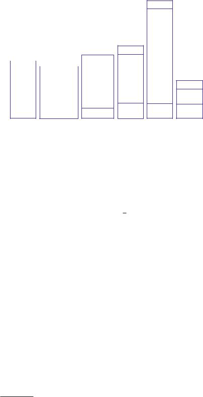
Classes. A class contains attributes (variables) and methods. A first rough overview of a class can be to just list the attributes and methods in a UML diagram as we have done in Figure 7.4 on page 393 for some of the key classes in the present chapter.

Below is a sample class with three attributes (m, M, and G) and three methods (a constructor, force, and visualize). The class represents the gravity force between two masses. This force is computed by the force method, while the visualize method plots the force as a function of the distance between the masses.

class Gravity:

"""Gravity force between two physical objects."""

def __init__(self, m, M):

def force(self, r):

G, m, M = self.G, self.m, self.M return G*m*M/r**2

def visualize(self, r_start, r_stop, n=100): from scitools.std import plot, linspace r = linspace(r_start, r_stop, n)

g = self.force(r)

title=’Gravity force: m=%g, M=%g’ % (self.m, self.M) plot(r, g, title=title)

Note that to access attributes inside the force method, and to call the force method inside the visualize method, we must prefix with self. Also recall that all methods must take self, “this” instance, as first argument, but the argument is left out in calls. The assignment of attributes to a local variable (e.g., G = self.G) inside methods is not necessary, but here it makes the mathematical formula easier to read and compare with standard mathematical notation.

This class (found in file Gravity.py) can be used to find the gravity force between the moon and the earth:

mass_moon = 7.35E+22; mass_earth = 5.97E+24 gravity = Gravity(mass_moon, mass_earth)

r = 3.85E+8 # earth-moon distance in meters Fg = gravity.force(r)

print ’force:’, Fg

Special Methods. A collection of special methods, with two leading and trailing underscores in the method names, o ers special syntax in Python programs. Table 7.1 on page 392 provides an overview of the most important special methods.

Table 7.1 Summary of some important special methods in classes. a and b are instances of the class whose name we set to A.

7.8.2 Summarizing Example: Interval Arithmetics

Input data to mathematical formulas are often subject to uncertainty, usually because physical measurements of many quantities involve measurement errors, or because it is di cult to measure a parameter and one is forced to make a qualified guess of the value instead. In such cases it could be more natural to specify an input parameter by an interval [a, b], which is guaranteed to contain the true value of the parameter. The size of the interval expresses the uncertainty in this parameter. Suppose all input parameters are specified as intervals, what will be the interval, i.e., the uncertainty, of the output data from the formula? This section develops a tool for computing this output uncertainty in

1.p + q = [a + c, b + d]

2.p − q = [a − d, b − c]

3.pq = [min(ac, ad, bc, bd), max(ac, ad, bc, bd)]

4.p/q = [min(a/c, a/d, b/c, b/d), max(a/c, a/d, b/c, b/d)] provided that [c, d] does not contain zero

For doing these calculations in a program, it would be natural to have a new type for quantities specified by intervals. This new type should support the operators +, -, *, and / according to the rules above. The task is hence to implement a class for interval arithmetics with special methods for the listed operators. Using the class, we should be able to estimate the uncertainty of two formulas:

1. The acceleration of gravity, g = 2y0T −2, given a 2% uncertainty in y0: y0 = [0.99, 1.01], and a 10% uncertainty in T : T = [Tm ·0.95, Tm · 1.05], with Tm = 0.45.

2.The volume of a sphere, V = 43 πR3, given a 20% uncertainty in R: R = [Rm · 0.9, Rm · 1.1], with Rm = 6.

Solution. The new type is naturally realized as a class IntervalMath whose data consist of the lower and upper bound of the interval. Special methods are used to implement arithmetic operations and printing of the object. Having understood class Vec2D from Chapter 7.5, it should be straightforward to understand the class below:

class IntervalMath:

def __init__(self, lower, upper): self.lo = float(lower) self.up = float(upper)

def __add__(self, other):

a, b, c, d = self.lo, self.up, other.lo, other.up return IntervalMath(a + c, b + d)

def __sub__(self, other):

a, b, c, d = self.lo, self.up, other.lo, other.up return IntervalMath(a - d, b - c)

def __mul__(self, other):

a, b, c, d = self.lo, self.up, other.lo, other.up

return IntervalMath(min(a*c, a*d, b*c, b*d), max(a*c, a*d, b*c, b*d))

def __div__(self, other):

a, b, c, d = self.lo, self.up, other.lo, other.up

# [c,d] cannot contain zero: if c*d <= 0:

raise ValueError\

(’Interval %s cannot be denominator because ’\ ’it contains zero’)

return IntervalMath(min(a/c, a/d, b/c, b/d), max(a/c, a/d, b/c, b/d))

def __str__(self):

return ’[%g, %g]’ % (self.lo, self.up)

The code of this class is found in the file IntervalMath.py. A quick demo of the class can go as

I = IntervalMath a = I(-3,-2)

b = I(4,5)

expr = ’a+b’, ’a-b’, ’a*b’, ’a/b’ for e in expr:

print ’%s =’ % e, eval(e)

The output becomes

a+b = [1, 3] a-b = [-8, -6] a*b = [-15, -8]

a/b = [-0.75, -0.4]

This gives the impression that with very short code we can provide a new type that enables computations with interval arithmetics and thereby with uncertain quantities. However, the class above has severe limitations as shown next.

Consider computing the uncertainty of aq if a is expressed as an interval [4, 5] and q is a number (float):

a = I(4,5) q = 2

b = a*q

This does not work so well:

File "IntervalMath.py", line 15, in __mul__

a, b, c, d = self.lo, self.up, other.lo, other.up AttributeError: ’float’ object has no attribute ’lo’

The problem is that a*q is a multiplication between an IntervalMath object a and a float object q. The __mul__ method in class IntervalMath is invoked, but the code there tries to extract the lo attribute of q, which does not exist since q is a float.

We can extend the __mul__ method and the other methods for arithmetic operations to allow for a number as operand – we just convert the number to an interval with the same lower and upper bounds:

def __mul__(self, other):

if isinstance(other, (int, float)): other = IntervalMath(other, other)

a, b, c, d = self.lo, self.up, other.lo, other.up return IntervalMath(min(a*c, a*d, b*c, b*d),

max(a*c, a*d, b*c, b*d))

Looking at the formula g = 2y0T −2, we run into a related problem: now we want to multiply 2 (int) with y0, and if y0 is an interval, this multiplication is not defined among int objects. To handle this case, we need to implement an __rmul__(self, other) method for doing other*self, as explained in Chapter 7.6.4:

396 7 Introduction to Classes

def __rmul__(self, other):

if isinstance(other, (int, float)):

other = IntervalMath(other, other) return other*self

Similar methods for addition, subtraction, and division must also be included in the class.

Returning to g = 2y0T −2, we also have a problem with T −2 when T is an interval. The expression T**(-2) invokes the power operator (at least if we do not rewrite the expression as 1/(T*T)), which requires a __pow__ method in class IntervalMath. We limit the possibility to have integer powers, since this is easy to compute by repeated multiplications:

def __pow__(self, exponent):

if isinstance(exponent, int): p = 1

if exponent > 0:

for i in range(exponent): p = p*self

elif exponent < 0:

for i in range(-exponent): p = p*self

p = 1/p

else: # exponent == 0

p = IntervalMath(1, 1) return p

else:

raise TypeError(’exponent must int’)

Another natural extension of the class is the possibility to convert an interval to a number by choosing the midpoint of the interval:

>>>a = IntervalMath(5,7)

>>>float(a)

6

float(a) calls a.__float__(), which we implement as

def __float__(self):

return 0.5*(self.lo + self.up)

A __repr__ method returning the right syntax for recreating the present instance is also natural to include in any class:

def __repr__(self):

return ’%s(%g, %g)’ % \

(self.__class__.__name__, self.lo, self.up)

We are now in a position to test out the extended class

IntervalMath.

>>>T = I(Tm*0.95, Tm*1.05) # 10% uncertainty

>>>print T

398 7 Introduction to Classes

Exercise 7.2. Make a very simple class.

Make a class Simple with one attribute i, one method double, which replaces the value of i by i+i, and a constructor that initializes the attribute. Try out the following code for testing the class:

s1 = Simple(4) for i in range(4):

s1.double() print s1.i

s2 = Simple(’Hello’) s2.double(); s2.double() print s2.i

s2.i = 100 print s2.i

Before you run this code, convince yourself what the output of the print statements will be. Name of program file: Simple.py.

Exercise 7.3. Extend the class from Ch. 7.2.1.

Add an attribute transactions to the Account class from Chapter 7.2.1. The new attribute counts the number of transactions done in the deposit and withdraw methods. The total number of transactions should be printed in the dump method. Write a simple test program to demonstrate that transaction gets the right value after some calls to deposit and withdraw. Name of program file: Account2.py.

Exercise 7.4. Make classes for a rectangle and a triangle.

The purpose of this exercise is to create classes like class Circle from Chapter 7.2.3 for representing other geometric figures: a rectangle with width W , height H, and lower left corner (x0, y0); and a general triangle specified by its three vertices (x0, y0), (x1, y1), and (x2, y2) as explained in Exercise 2.17. Provide three methods: __init__ (to initialize the geometric data), area, and circumference. Name of program file: geometric_shapes.py.

Exercise 7.5. Make a class for straight lines.

Make a class Line whose constructor takes two points p1 and p2 (2- tuples or 2-lists) as input. The line goes through these two points (see function line in Chapter 2.2.7 for the relevant formula of the line). A value(x) method computes a value on the line at the point x. Here is a demo in an interactive session:

>>>from Line import Line

>>>line = Line((0,-1), (2,4))

>>>print line.value(0.5), line.value(0), line.value(1) 0.25 -1.0 1.5

Name of program file: Line.py.

Exercise 7.6. Improve the constructor in Exer. 7.5.

The constructor in class Line in Exercise 7.5 takes two points as arguments. Now we want to have more flexibility in the way we specify

a straight line: we can give two points, a point and a slope, or a slope and the line’s interception with the y axis. Hint: Let the constructor take two arguments p1 and p2 as before, and test with isinstance whether the arguments are float or tuple/list to determine what kind of data the user supplies:

if isinstance(p1, (tuple,list)) and isinstance(p2, (float,int)):

Exercise 7.7. Make a class for quadratic functions.

Consider a quadratic function f (x; a, b, c) = ax2 + bx + c. Make a class Quadratic for representing f , where a, b, and c are attributes, and the methods are

1.value for computing a value of f at a point x,

2.table for writing out a table of x and f values for n x values in the interval [L, R],

3.roots for computing the two roots.

Name of program file: Quadratic.py.

Exercise 7.8. Make a class for linear springs.

To elongate a spring a distance x, one needs to pull the spring with a force kx. The parameter k is known as the spring constant. The corresponding potential energy in the spring is 12 kx2.

Make a class for springs. Let the constructor store k as a class attribute, and implement the methods force(x) and energy(x) for evaluating the force and the potential energy, respectively.

The following function prints a table of function values for an arbitrary mathematical function f(x). Demonstrate that you can send the force and energy methods as the f argument to table.

def table(f, a, b, n, heading=’’):

"""Write out f(x) for x in [a,b] with steps h=(b-a)/n.""" print heading

h = (b-a)/float(n) for i in range(n+1): x = a + i*h

print ’function value = %10.4f at x = %g’ % (f(x), x)

Name of program file: Spring.py.

Exercise 7.9. Implement Lagrange’s interpolation formula.

Given n + 1 points (x0, y0), (x1, y1), . . . , (xn, yn), the following polynomial of degree n goes through all the points:

k=0