primer_on_scientific_programming_with_python

The output 3-tuple holds the approximation to a root, the number of iterations, and the value of f at the approximate root (a measure of the error in the equation).

The exact root is 1.1, and the convergence toward this value is very slow6 (for example, an epsilon tolerance of 10−10 requires 18 iterations with an error of 10−3). Using an exact derivative gives almost the same result:

>>> def df_exact(x):

... return 100000*(2*(x-0.9)*(x-1.1)**3 + \

... (x-0.9)**2*3*(x-1.1)**2)

...

>>> Newton(f, 1.01, df_exact, epsilon=1E-5) (1.0987610065618421, 8, -7.5139689100699629e-06)

This example indicates that there are hardly any drawbacks in using a “smart” inexact general di erentiation approach as in the Derivative class. The advantages are many – most notably, Derivative avoids potential errors from possibly incorrect manual coding of possibly lengthy expressions of possibly wrong hand-calculations. The errors in the involved approximations can be made smaller, usually much smaller than other errors, like the tolerance in Newton’s method in this example or the uncertainty in physical parameters in real-life problems.

7.3.3 Example: Automagic Integration

We can apply the ideas from Chapter 7.3.2 to make a class for computing the integral of a function numerically. Given a function f (x), we want to compute

x

F (x; a) = f (t)dt .

a

The computational technique consists of using the Trapezoidal rule with n intervals (n + 1 points):

where h = (x − a)/n. In an application program, we want to compute F (x; a) by a simple syntax like

def f(x):

return exp(-x**2)*sin(10*x)

6Newton’s method converges very slowly when the derivative of f is zero at the roots of f . Even slower convergence appears when higher-order derivatives also are zero, like in this example. Notice that the error in x is much larger than the error in the equation (epsilon).

a = 0; n = 200

F = Integral(f, a, n) print F(x)

Here, f(x) is the Python function to be integrated, and F(x) behaves as a Python function that calculates values of F (x; a).

A Simple Implementation. Consider a straightforward implementation of the Trapezoidal rule in a Python function:

def trapezoidal(f, a, x, n): h = (x-a)/float(n)

I = 0.5*f(a)

for i in iseq(1, n-1):

I += f(a + i*h) I += 0.5*f(x)

I *= h return I

The iseq function is an alternative to range where the upper limit is included in the set of numbers (see Chapters 4.3.1 and 4.5.6). We can alternatively use range(1, n), but the correspondence with the indices in the mathematical description of the rule is then not completely direct. The iseq function is contained in scitools.std, so if you make a “star import” from this module, you have iseq available.

Class Integral must have some attributes and a __call__ method. Since the latter method is supposed to take x as argument, the other parameters a, f, and n must be class attributes. The implementation then becomes

class Integral:

def __init__(self, f, a, n=100): self.f, self.a, self.n = f, a, n

def __call__(self, x):

return trapezoidal(self.f, self.a, x, self.n)

Observe that we just reuse the trapezoidal function to perform the calculation. We could alternatively have copied the body of the trapezoidal function into the __call__ method. However, if we already have this algorithm implemented and tested as a function, it is better to call the function. The class is then known as a wrapper of the underlying function. A wrapper allows something to be called with alternative syntax. With the Integral(x) wrapper we can supply the upper limit of the integral only – the other parameters are supplied when we create an instance of the Integral class.

An application program computing 2π sin x dx might look as fol-

0

lows:

from math import sin, pi

G = Integral(sin, 0, 200) value = G(2*pi)

>>>y = Y(1.5)

>>>y(0.2)

0.1038

>>>print y

v0*t - 0.5*g*t**2; v0=1.5

What have we gained by using special methods? Well, we can still only evaluate the formula and write it out, but many users of the class will claim that the syntax is more attractive since y(t) in code means y(t) in mathematics, and we can do a print y to view the formula. The bottom line of using special methods is to achieve a more user-friendly syntax. The next sections illustrate this point further.

7.3.5 Example: Phone Book with Special Methods

Let us reconsider class Person from Chapter 7.2.2. The dump method in that class is better implemented as a __str__ special method. This is easy: We just change the method name and replace print s by return s.

Storing Person instances in a dictionary to form a phone book is straightforward. However, we make the dictionary a bit easier to use if we wrap a class around it. That is, we make a class PhoneBook which holds the dictionary as an attribute. An add method can be used to add a new person:

class PhoneBook:

def __init__(self):

self.contacts = {} # dict of Person instances

def add(self, name, mobile=None, office=None, private=None, email=None):

p = Person(name, mobile, office, private, email) self.contacts[name] = p

A __str__ can print the phone book in alphabetic order:

def __str__(self): s = ’’

for p in sorted(self.contacts): s += str(self.contacts[p])

return s

To retrieve a Person instance, we use the __call__ with the person’s name as argument:

def __call__(self, name):

return self.contacts[name]

The only advantage of this method is simpler syntax: For a PhoneBook b we can get data about NN by calling b(’NN’) rather than accessing the internal dictionary b.contacts[’NN’].

We can make a simple test function for a phone book with three names:

b = PhoneBook()

b.add(’Ole Olsen’, office=’767828292’, email=’olsen@somemail.net’)

b.add(’Hans Hanson’,

office=’767828283’, mobile=’995320221’) b.add(’Per Person’, mobile=’906849781’) print b(’Per Person’)

print b

The output becomes

Per Person

mobile phone: 906849781

Hans Hanson

mobile phone: 995320221 office phone: 767828283

Ole Olsen

office phone: 767828292

email address: olsen@somemail.net

Per Person

mobile phone: 906849781

You are strongly encouraged to work through this last demo program by hand and simulate what the program does. That is, jump around in the code and write down on a piece of paper what various variables contain after each statement. This is an important and good exercise! You enjoy the happiness of mastering classes if you get the same output as above. The complete program with classes Person and PhoneBook and the test above is found in the file phone_book.py. You can run this program, statement by statement, in a debugger (see Appendix D.1) to control that your understanding of the program flow is correct.

Remark. Note that the names are sorted with respect to the first names. The reason is that strings are sorted after the first character, then the second character, and so on. We can supply our own tailored sort function, as explained in Exercise 2.44. One possibility is to split the name into words and use the last word for sorting:

def last_name_sort(name1, name2): lastname1 = name1.split()[-1] lastname2 = name2.split()[-1] if lastname1 < lastname2:

return -1

elif lastname1 > lastname2:

return 1 else: # equality

return 0

for p in sorted(self.contacts, last_name_sort):

...

7.3.6 Adding Objects

Let a and b be instances of some class C. Does it make sense to write a + b? Yes, this makes sense if class C has defined a special method

__add__:

class C:

...

__add__(self, other):

...

The __add__ method should add the instances self and other and return the result as an instance. So when Python encounters a + b, it will check if class C has an __add__ method and interpret a + b as the call a.__add__(b). The next example will hopefully clarify what this idea can be used for.

7.3.7 Example: Class for Polynomials

Let us create a class Polynomial for polynomials. The coe cients in the polynomial can be given to the constructor as a list. Index number i in this list represents the coe cients of the xi term in the polynomial. That is, writing Polynomial([1,0,-1,2]) defines a polynomial

1 + 0 · x − 1 · x2 + 2 · x3 = 1 − x2 + 2x3 .

Polynomials can be added (by just adding the coe cients) so our class may have an __add__ method. A __call__ method is natural for evaluating the polynomial, given a value of x. The class is listed below and explained afterwards.

class Polynomial:

def __init__(self, coefficients): self.coeff = coefficients

def __call__(self, x): s = 0

for i in range(len(self.coeff)): s += self.coeff[i]*x**i

return s

def __add__(self, other):

# start with the longest list and add in the other: if len(self.coeff) > len(other.coeff):

sum_coeff = self.coeff[:] # copy! for i in range(len(other.coeff)): sum_coeff[i] += other.coeff[i]

else:

sum_coeff = other.coeff[:] # copy! for i in range(len(self.coeff)):

sum_coeff[i] += self.coeff[i] return Polynomial(sum_coeff)

366 7 Introduction to Classes

Implementation. Class Polynomial has one attribute: the list of coefficients. To evaluate the polynomial, we just sum up coe cient no. i times xi for i = 0 to the number of coe cients in the list.

The __add__ method looks more advanced. The idea is to add the two lists of coe cients. However, it may happen that the lists are of unequal length. We therefore start with the longest list and add in the other list, element by element. Observe that sum_coeff starts out as a copy of self.coeff: If not, changes in sum_coeff as we compute the sum will be reflected in self.coeff. This means that self would be the sum of itself and the other instance, or in other words, adding two instances, p1+p2, changes p1 – this is not what we want! An alternative implementation of class Polynomial is found in Exercise 7.32.

A subtraction method __sub__ can be implemented along the lines of __add__, but is slightly more complicated and left to the reader through Exercise 7.33. A somewhat more complicated operation, from a mathematical point of view, is the multiplication of two polynomials.

The double sum must be implemented as a double loop, but first the list for the resulting polynomial must be created with length M +N +1 (the highest exponent is M + N and then we need a constant term). The implementation of the multiplication operator becomes

def __mul__(self, other): c = self.coeff

d = other.coeff M = len(c) - 1 N = len(d) - 1

result_coeff = zeros(M+N-1) for i in range(0, M+1):

for j in range(0, N+1): result_coeff[i+j] += c[i]*d[j]

return Polynomial(result_coeff)

We could also include a method for di erentiating the polynomial according to the formula

If ci is stored as a list c, the list representation of the derivative, say its name is dc, fulfills dc[i-1] = i*c[i] for i running from 1 to the largest index in c. Note that dc has one element less than c.

There are two di erent ways of implementing the di erentiation functionality, either by changing the polynomial coe cients, or by re-

turning a new Polynomial instance from the method such that the original polynomial instance is intact. We let p.differentiate() be an implementation of the first approach, i.e., this method does not return anything, but the coe cients in the Polynomial instance p are altered. The other approach is implemented by p.derivative(), which returns a new Polynomial object with coe cients corresponding to the derivative of p.

The complete implementation of the two methods is given below:

def differentiate(self):

"""Differentiate this polynomial in-place.""" for i in range(1, len(self.coeff)):

self.coeff[i-1] = i*self.coeff[i] del self.coeff[-1]

def derivative(self):

"""Copy this polynomial and return its derivative.""" dpdx = Polynomial(self.coeff[:]) # make a copy dpdx.differentiate()

return dpdx

The Polynomial class with a differentiate method and not a derivative method would be mutable (see Chapter 6.2.3) and allow in-place changes of the data, while the Polynomial class with derivative and not differentiate would yield an immutable object where the polynomial initialized in the constructor is never altered7.

out differentiate, its function body must of course be copied into derivative since derivative now relies on that code). However, since the main purpose of this class is to illustrate various types of programming techniques, we keep both versions.

Usage. As a demonstration of the functionality of class Polynomial, we introduce the two polynomials

p1(x) = 1 − x, p2(x) = x − 6x4 − x5 .

>>>p1 = Polynomial([1, -1])

>>>p2 = Polynomial([0, 1, 0, 0, -6, -1])

>>>p3 = p1 + p2

>>>print p3.coeff

[1, 0, 0, 0, -6, -1]

>>>p4 = p1*p2

>>>print p4.coeff

[0, 1, -1, 0, -6, 5, 1]

>>> p5 = p2.derivative()

7Technically, it is possible to grab the coeff variable in a class instance and alter this list. By starting coeff with an underscore, a Python programming convention tells programmers that this variable is for internal use in the class only, and not to be altered by users of the instance, see Chapters 7.2.1 and 7.6.2.

>>> print p5.coeff [1, 0, 0, -24, -5]

One verification of the implementation may be to compare p3 at (e.g.)

x= 1/2 with p1(x) + p2(x):

>>>x = 0.5

>>>p1_plus_p2_value = p1(x) + p2(x)

>>>p3_value = p3(x)

>>>print p1_plus_p2_value - p3_value

0.0

Note that p1 + p2 is very di erent from p1(x) + p2(x). In the former case, we add two instances of class Polynomial, while in the latter case we add two instances of class float (since p1(x) and p2(x) imply calling __call__ and that method returns a float object).

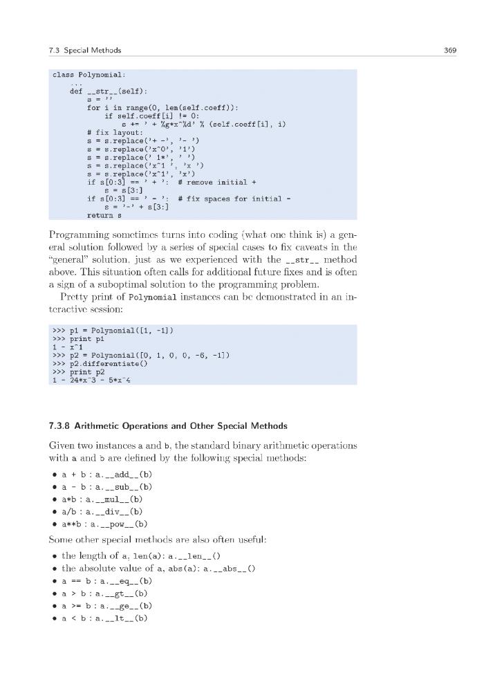
Pretty Print of Polynomials. The Polynomial class can also be equipped with a __str__ method for printing the polynomial to the screen. A first, rough implementation could simply add up strings of the form

+ self.coeff[i]*x^i:

class Polynomial:

...

def __str__(self): s = ’’

for i in range(len(self.coeff)):

s += ’ + %g*x^%d’ % (self.coeff[i], i) return s

However, this implementation leads to ugly output from a mathematical viewpoint. For instance, a polynomial with coe cients

[1,0,0,-1,-6] gets printed as

+ 1*x^0 + 0*x^1 + 0*x^2 + -1*x^3 + -6*x^4

A more desired output would be

1 - x^3 - 6*x^4

That is, terms with a zero coe cient should be dropped; a part ’+ -’ of the output string should be replaced by ’- ’; unit coe cients should be dropped, i.e., ’ 1*’ should be replaced by space ’ ’; unit power should be dropped by replacing ’x^1 ’ by ’x ’; zero power should be dropped and replaced by 1, initial spaces should be fixed, etc. These adjustments can be implemented using the replace method in string objects and by composing slices of the strings. The new version of the __str__ method below contains the necessary adjustments. If you find this type of string manipulation tricky and di cult to understand, you may safely skip further inspection of the improved __str__ code since the details are not essential for your present learning about the class concept and special methods.