primer_on_scientific_programming_with_python

A = 1; a = 0.1 dg = diff(g, 1.5)

The use of global variables is in general considered bad programming. Why global variables are problematic in the present case can be illustrated when there is need to work with several versions of a function. Suppose we want to work with two versions of y(t; v0), one with v0 = 1 and one with v0 = 5. Every time we call y we must remember which version of the function we work with, and set v0 accordingly prior to the call:

v0 = 1; r1 = y(t)

v0 = 5; r2 = y(t)

Another problem is that variables with simple names like v0, a, and A may easily be used as global variables in other parts of the program. These parts may change our v0 in a context di erent from the y function, but the change a ects the correctness of the y function. In such a case, we say that changing v0 has side e ects, i.e., the change a ects other parts of the program in an unintentional way. This is one reason why a golden rule of programming tells us to limit the use of global variables as much as possible.

Another solution to the problem of needing two v0 parameters could be to introduce two y functions, each with a distinct v0 parameter:

def y1(t): g = 9.81

return v0_1*t - 0.5*g*t**2

def y2(t): g = 9.81

return v0_2*t - 0.5*g*t**2

Now we need to initialize v0_1 and v0_2 once, and then we can work with y1 and y2. However, if we need 100 v0 parameters, we need 100 functions. This is tedious to code, error prone, di cult to administer, and simply a really bad solution to a programming problem.

So, is there a good remedy? The answer is yes: The class concept solves all the problems described above!

7.1.2 Representing a Function as a Class

A class contains a set of variables (data) and a set of functions, held together as one unit. The variables are visible in all the functions in the class. That is, we can view the variables as “global” in these functions. These characteristics also apply to modules, and modules can be used to obtain many of the same advantages as classes o er (see comments

in Chapter 7.1.5). However, classes are technically very di erent from modules. You can also make many copies of a class, while there can be only one copy of a module. When you master both modules and classes, you will clearly see the similarities and di erences. Now we continue with a specific example of a class.

Consider the function y(t; v0) = v0t − 12 gt2. We may say that v0 and g, represented by the variables v0 and g, constitute the data. A Python function, say value(t), is needed to compute the value of y(t; v0) and this function must have access to the data v0 and g, while t is an argument.

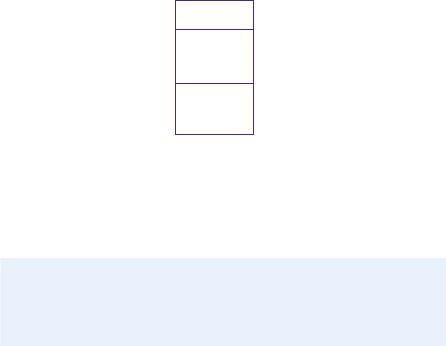
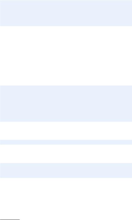
A programmer experienced with classes will then suggest to collect the data v0 and g, and the function value(t), together as a class. In addition, a class usually has another function, called constructor for initializing the data. The constructor is always named __init__. Every class must have a name, often starting with a capital, so we choose Y as the name since the class represents a mathematical function with name y. Figure 7.1 sketches the contents of class Y as a so-called UML diagram, here created with Lumpy (from Appendix E.3) with aid of the little program class_Y_v1_UML.py. The UML diagram has two “boxes”, one where the functions are listed, and one where the variables are listed. Our next step is to implement this class in Python.

Y

__init__ value

g v0

Fig. 7.1 UML diagram with function and data in the simple class Y for representing a mathematical function y(t; v0).

Implementation. The complete code for our class Y looks as follows in Python:

class Y:

def __init__(self, v0): self.v0 = v0 self.g = 9.81

def value(self, t):

return self.v0*t - 0.5*self.g*t**2

A puzzlement for newcomers to Python classes is the self parameter, which may take some e orts and time to fully understand.

It takes some time to understand the self variable, but more examples and hands-on experience with class programming will help, so just be patient and continue reading.

Extension of the Class. We can have as many attributes and methods as we like in a class, so let us add a new method to class Y. This method is called formula and prints a string containing the formula of the mathematical function y. After this formula, we provide the value of v0. The string can then be constructed as

’v0*t - 0.5*g*t**2; v0=%g’ % self.v0

where self is an instance of class Y. A call of formula does not need any arguments:

print y.formula()

should be enough to create, return, and print the string. However, even if the formula method does not need any arguments, it must have a self argument, which is left out in the call but needed inside the method to access the attributes. The implementation of the method is therefore

def formula(self):

return ’v0*t - 0.5*g*t**2; v0=%g’ % self.v0

For completeness, the whole class now reads

class Y:

def __init__(self, v0): self.v0 = v0 self.g = 9.81

def value(self, t):

return self.v0*t - 0.5*self.g*t**2

def formula(self):

return ’v0*t - 0.5*g*t**2; v0=%g’ % self.v0

Example on use may be

y = Y(5) t = 0.2

v = y.value(t)

print ’y(t=%g; v0=%g) = %g’ % (t, y.v0, v) print y.formula()

with the output

y(t=0.2; v0=5) = 0.8038 v0*t - 0.5*g*t**2; v0=5

Remark. A common mistake done by newcomers to the class construction is to place the code that applies the class at the same indentation as the class methods. This is illegal. Only method definitions and assignments to so-called static attributes (Chapter 7.7) can appear in

the indented block under the class headline. Ordinary attribute assignment must be done inside methods. The main program using the class must appear with the same indent as the class headline.

Using Methods as Ordinary Functions. We may create several y functions with di erent values of v0:

We can treat y1.value, y2.value, and y3.value as ordinary Python functions of t, and then pass them on to any Python function that expects a function of one variable. In particular, we can send the functions to the diff(f, x) function from page 339:

dy1dt = diff(y1.value, 0.1) dy2dt = diff(y2.value, 0.1) dy3dt = diff(y3.value, 0.2)

Inside the diff(f, x) function, the argument f now behaves as a function of one variable that automatically carries with it two variables v0 and g. When f refers to (e.g.) y3.value, Python actually knows that f(x) means y3.value(x), and inside the y3.value method self is y3, and we have access to y3.v0 and y3.g.

Doc Strings. A function may have a doc string right after the function definition, see Chapter 2.2.7. The aim of the doc string is to explain the purpose of the function and, for instance, what the arguments and return values are. A class can also have a doc string, it is just the first string that appears right after the class headline. The convention is to enclose the doc string in triple double quotes """:

class Y:

"""The vertical motion of a ball."""

def __init__(self, v0):

...

More comprehensive information can include the methods and how the class is used in an interactive session:

class Y:

"""

Mathematical function for the vertical motion of a ball.

Methods:

constructor(v0): set initial velocity v0.

value(t): compute the height as function of t. formula(): print out the formula for the height.

Attributes:

v0: the initial velocity of the ball (time 0). g: acceleration of gravity (fixed).

Usage:

>>>y = Y(3)

>>>position1 = y.value(0.1)

>>>position2 = y.value(0.3)

>>>print y.formula()

v0*t - 0.5*g*t**2; v0=3

"""

7.1.3 Another Function Class Example

Let us apply the ideas from the Y class to the v(r) function specified in (4.20) on page 230. We may write this function as v(r; β, μ0, n, R) to indicate that there is one primary independent variable (r) and four physical parameters (β, μ0, n, and R). The class typically holds the physical parameters as variables and provides an value(r) method for computing the v function:

class VelocityProfile:

def __init__(self, beta, mu0, n, R):

self.beta, self.mu0, self.n, self.R = beta, mu0, n, R

def value(self, r):

beta, mu0, n, R = self.beta, self.mu0, self.n, self.R n = float(n) # ensure float divisions

v = (beta/(2.0*mu0))**(1/n)*(n/(n+1))*\ (R**(1+1/n) - r**(1+1/n))

return v

There is seemingly one new thing here in that we initialize several variables on the same line4:

self.beta, self.mu0, self.n, self.R = beta, mu0, n, R

This is perfectly valid Python code and equivalent to the multi-line code

self.beta = beta self.mu0 = mu0

self.n = n self.R = R

In the value method it is convenient to avoid the self. prefix in the mathematical formulas and instead introduce the local short names beta, mu0, n, and R. This is in general a good idea, because it makes it easier to read the implementation of the formula and check its correctness.

Here is one possible application of class VelocityProfile:

4The comma-separated list of variables on the right-hand side forms a tuple so this assignment is just the usual construction where a set of variables on the left-hand side is set equal to a list or tuple on the right-hand side, element by element. See page 58.