диафрагмированные волноводные фильтры / d0b6eab4-ee66-48f9-8028-3068c251b6eb

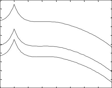
Figure 3.3 Choices of materials and of technology for different characteristics of filters

Table 3.3 Performance of SAW filters

32

CHAPTER 4

THEORY AND DESIGN

4.1Introduction

Designing a pulse FMCW radar is a complicated task which involves many variables concerning maximum detectable range, relative velocity, noise considerations, necessary transmitter power and the final interpretation of the received information. Of course, some of these variables are constrains regarding to the application requirements of the system and some of the variables are to be defined after the

meters. The radar must be designed to have the maximum detectable range longer than 1000 meters. Target in the system is an infinite obstacle and stationary. Small size and lightweight is also the primary requirements.

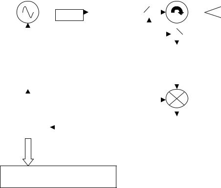
Throughout this chapter some design issues are given and a simplified test technique for the radar system using surface acoustic wave (SAW) devices is given as well. The block diagram of the FMCW radar has already been given in Figure (2.5). Block diagram for pulse FMCW radar is given in Figure (4.1).

33

Data Acquisition Systems

(Computer, Display, VTR)

Figure 4.1 Pulse FMCW radar block diagram

4.2Back Scattering From Target

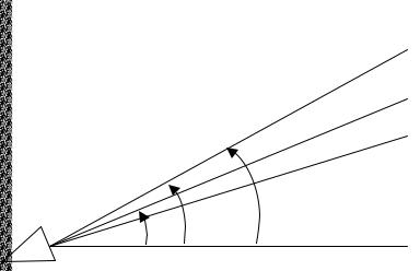
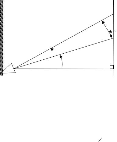
The system will be able to measure the distance of the targets within 1000 meters range. The target is the earth’s surface. The radar itself can rotate both on the and axes of the spherical coordinate system but rotation is limited to 90 degrees on the axis. However, ground surface extends to infinity in dimension compared to the illumination area of the radar. Thus, rotation on the axis does not affect the illuminated area of the target by radar which has a uniform beamwidth on the and axes. Radar and target can be seen in the Figure (4.2).

34

The azimuth beamwidth along R is denoted by B and the azimuth beamwidths along the cuts 0+ B/2 and 0- B/2 are 1 and 2, also assumed to be equal ( 1 = 2 = B). To calculate the power related issues we must define the illuminated area

( S) with respect to angle of incidence ( ), beamwidth of

the antenna ( B) and distance from target (d). The illuminated area by the radar ( S) can be calculated from Equation (4.1).

Received power at the antenna port ( Pr), by the reflections of the transmitted signal from the illuminated surface of the target ( S), can be expressed by Equation (4.2)

35

R1

d

Radar

Target

Figure 4.3 Illuminated area

Radar Cross Section (RCS) of the target can be approximated as an exponential function given in Equation (4.4) [10]

o is called the radar land reflectivity. o is usually expressed in dB(m2/m2). o has a strong dependency to the type of the surface (roughness) especially for the lower microwave frequencies and vary between -3 dB to -29 dB for grazing angles 7 to 70o. The median value is -14 dB which is the average of the various resulted from experiment. For the grazing angles greater than 65o, o so does o rapidly increases to a value of 0 to 15 dB (m2/m2). The maximum values are dominant for the urban areas. Land reflectivity

incidence = 0o and falls off rapidly as the increases [10].

The gain pattern of the antenna with gain G can be

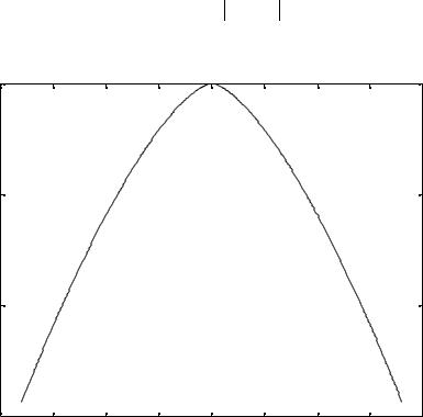
fn (θ) is the normalized antenna pattern in elevation plane and can be approximated by a Gaussian function normalized to 0 dB. Normalized antenna pattern equals to -3 dB in Equation [4.6] when is equal to half of the beamwidth.

(Degrees)

Figure 4.4 Normalized antenna field pattern

37

Substituting Equation (4.1), (4.3), (4.5) in the Equation (4.2), the received echo power at the antenna port ( Pr) can be found as in Equation (4.7).

reflected from the target. Power received from an angle of incidence from an angular width of is;

4.3Echo Power Angular Distribution

Angular distribution (density) of the received echo

signal at the antenna of the system is plotted using Equation (4.10), changing from -10o to 70o for different Q values corresponding to distance of 100, 500 and 1000

meters. The MATLAB (version 6.5) “m files” necessary to plot the angular distribution are given in Appendix C. Two source

38

codes (m files) for MATLAB in Appendix C, calculates the angular distribution of the received echo for = 1o using two different techniques and results are very close to each other.

distribution of the received echo power (dBm) in =1o angular width.

Frequency range of the system is between 800-900 MHz and for the calculations of the angular distribution of the received echo power, center frequency is taken as 850 MHz. From Figure (4.5) we can conclude the received echo signal will be maximum -50 dBm and the minimum received signal will be approximately -100 dBm at grazing angle of 30 degrees. The rain and atmospheric attenuations can be neglected at this frequency [1]. The output power transmitted at the antenna (Pt) is taken as 30 dBm (1W) and the elevation and azimuth beamwidths of the antenna ( B, B) are taken as both 80o and the gain of the antenna (G) is taken as 8 dB.

39

Figure 4.5 Angular distribution of the echo power at the antenna port

4.3Echo Power Spectrum

Echo power spectrum of the radar determined by replacing the angular information with frequency information, which can be derived using Equation (2.11).

K is the ranging sensitivity in Hz/m.

R is the change in the radial distance when the angle

of incidence is change by . From Figure (4.3);