


2
SENSOR DEPLOYMENT, SELF-ORGANIZATION, AND LOCALIZATION
2.1 INTRODUCTION
A key attribute of sensor networks is to be able to self-form, that is, when randomly deployed to be able to organize into an efficient network capable of gathering data in a useful and efficient manner. Often, gathering data in a useful manner requires that the exact location of a sensor be known. This requires that sensors be able to determine their location. This location information is often reused for other purposes. For example, once sensors know their location, and that of their neighbors, redundant sensors can be powered down to save energy. Likewise, low-energy communication paths may be established between nodes. Coverage holes in the sensor network may be uncovered and, through mobility, healed. In this chapter we address issues of network formation, including localization.
Sensor positioning problems are a critical area of research for sensor network operations. Sensor networks are useless if their configurations are not robust to power degradation or they are prone to breach by the very objects they are designed to detect. Many distributed algorithms rely on sensors with accurate knowledge of their position. While this can be achieved by providing each sensor with a Global Positioning System (GPS) unit, this is not always possible or desirable. Hence, internal localization algorithms are required. This chapter explores the issues of sensor placement for robust and scalable target detection and sensor node localization over large distances.
Section 2.2 by Sabbineni and Chakrabarty describes a fully distributed algorithm for exploiting redundancy in sensor networks to maintain connectivity and coverage in response to power degradation. When active nodes fail due to energy depletion or other reasons such as wearout, SCARE replaces them appropriately with inactive nodes.
Section 2.3 by Ji and Zha studies some situations where most existing sensor positioning methods tend to fail to perform well. It then explores the idea of using dimensionality reduction to estimate sensors coordinates in space; a distributed sensor positioning method based on multidimensional scaling technique is proposed.
Sensor Network Operations, Edited by Phoha, LaPorta, and Griffin
Copyright C 2006 The Institute of Electrical and Electronics Engineers, Inc.
13
14 SENSOR DEPLOYMENT, SELF-ORGANIZATION, AND LOCALIZATION
The location estimation or localization problem in wireless sensor networks is to locate the sensor nodes based on ranging device measurements of the distances between node pairs. A distance is censored when the ranging devices are unreliable and the distance between transmitting and receiving nodes is large. Section 2.4 by Lee, Varaiya, and Sengupta compares several approaches for estimating censored distances with a proposed strategy called trigonometric k clustering.
Section 2.5 by Onur, Ersoy, and Deli¸c cedilla considers the sensing coverage area of surveillance wireless sensor networks. The sensing coverage is determined by applying the Neyman–Pearson detection model and defining the breach probability on a grid-modeled field. Weakest breach paths are determined using Dijkstra’s algorithm.
The discussions in this chapter enhance the state of the art in sensor network operations by presenting solutions to the problems of sensor placement and localization. These results can be used to prolong the life of deployed sensor networks, enhance the quality of service of perimeter networks, and provide introspection necessary for sensor localization in highly distributed networks.
2.2 SCARE: A SCALABLE SELF-CONFIGURATION AND ADAPTIVE RECONFIGURATION SCHEME FOR DENSE SENSOR NETWORKS
Harshavardhan Sabbineni and Krishnendu Chakrabarty
We present a distributed self-configuration and adaptive reconfiguration scheme for dense sensor networks. The proposed algorithm, termed self-configuration and adaptive reconfiguration (SCARE), distributes the set of nodes in the network into subsets of coordinator and noncoordinator nodes. Redundancy is exploited not only to maintain the coverage and connectivity provided by sensor deployment but also to prolong the network lifetime. When active nodes fail due to energy depletion or other reasons such as wearout, SCARE replaces them appropriately with inactive nodes. Simulation results demonstrate that SCARE outperforms the previously proposed Span method in terms of coverage, energy usage, and the average delay per message.
2.2.1 Background Information
Advances in miniaturization of microelectronic and mechanical structures (MEMS) have led to battery-powered sensor nodes that have sensing, communication, and processing capabilities [1, 2]. Wireless sensor networks are networks of large numbers of such sensor nodes. Example applications of such sensor networks include the monitoring of wildfires, inventory tracking, assembly line monitoring, and target tracking in military systems. Upon deployment in a remote or a hostile location, sensor nodes might fail with time due to loss of battery power, an enemy attack, or a change in environmental conditions. The replacement of each failed sensor node with a new sensor node is expensive and often infeasible, and it is therefore undesirable. Hence in such cases, a large number of redundant sensor nodes are deployed with the expectation that these nodes will be used later when some other nodes fail. The self-configuration of a large number of sensor nodes requires a distributed solution. In this section, we present a scalable self-configuration and an adaptive reconfiguration (SCARE) algorithm for distributed sensor networks.
2.2 SCARE |
15 |
An effective self-configuration scheme should have the following characteristics. It should be completely distributed and localized because a centralized solution is often not scalable for wireless sensor networks. It should be simple without excessive message overhead because sensor nodes typically have limited energy resources. It should be energyefficient and require only a small number of nodes to stay awake and perform multihop routing, and it should keep the other nodes in a sleep state.
We propose a solution that meets the above design requirements. We present a distributed self-configuration scheme that distributes the set of nodes in the sensor network into subsets of coordinator nodes and noncoordinator nodes. While coordinator nodes stay awake, provide coverage, and perform multihop routing in the network, noncoordinator nodes go to sleep. When nodes fail, SCARE adaptively reconfigures the network by selecting appropriate noncoordinator nodes to become coordinators and take over the role of failed coordinators. This scheme only needs local topology information and uses simple data structures in its implementation.
2.2.2 Relevant Prior Work
A number of topology management algorithms have been proposed for ad hoc and sensor networks [3–6]. While the connectivity problem has been studied in considerable detail for wireless ad hoc networks, less attention has been devoted to the problem of balancing connectivity and coverage. The GAF scheme [4] uses geographic location information of the sensor nodes, and it divides the network into fixed-size virtual square grids. GAF identifies redundant nodes within each virtual grid and switches off their radios to achieve energy savings. In contrast, SCARE achieves energy savings by selectively powering down some of the nodes that are within the sensing radius of a coordinator. A coverage-preserving node scheduling scheme is described in [7] that extends the LEACH [8] protocol to achieve energy savings. In this scheme, nodes advertise their position information in each round. Each node evaluates its eligibility to switch itself off by calculating its sensing area and comparing it with its neighbors’s. If a node’s sensing area is embraced by a union set of its neighbors’s, then it turns itself off. To prevent blind spots in coverage due to several eligible nodes switching themselves off simultaneously, a back-off-based scheduling is used. After the back-off interval has elapsed, nodes broadcast a status advertisement message to let other nodes know about their on/off status. Thus, each node broadcasts two messages in this scheme. In contrast, SCARE needs fewer than two messages per node on average during its operation. The scheme in [7] also utilizes location information of the nodes for its operation. SCARE only needs an estimate of the distance between the nodes.
The STEM scheme described in [6] trades off latency for energy savings by putting nodes aggressively to sleep and waking them up only when there is data to forward. It uses a second radio operating at a lower duty cycle for transmitting periodic beacons to wake up nodes when there is data to forward. SCARE does not use a separate paging channel for selfconfiguration. Nevertheless, SCARE can integrate well with STEM to achieve significant energy savings.
In AFECA [9], nodes listen to the channel for transmissions. AFECA conservatively tries to keep nodes awake when there are not too many neighbors in its radio range. In order to deduce this information, each node has to listen to transmissions that are not meant for it. In SCARE, however, nodes listen at only periodic intervals in order to determine their states.
16 SENSOR DEPLOYMENT, SELF-ORGANIZATION, AND LOCALIZATION
The PAMAS [10] multiaccess protocol saves power by switching off the radio of a node when it is not transmitting or receiving. This method saves power when idle listening consumes significantly less energy compared to message reception.
The Span approach [5] appears to be the most closely related to SCARE. Span attempts to save energy by switching off redundant nodes without losing the connectivity of the network. Nodes make decisions based on their local topology information. However, SCARE differs from Span in that it uses distance estimates to determine the state of a node. Span uses a communication mechanism to obtain this information. Since Span was developed for ad hoc networks, its main focus is on ensuring network connectivity through energyefficient topology management. It is not directed toward ensuring the sensing coverage of a given region. SCARE also differs from Span in that, in addition to ensuring network connectivity and low-energy self-configuration, it attempts to provide a high level of sensing coverage.
A TDMA-based self-organization scheme for sensor networks is presented in [11]. Each node uses a superframe, similar to a TDMA frame, to schedule different time slots for different neighbors. However, this scheme does not take advantage of the redundancy inherent in wireless sensor networks to power off some nodes.
SCARE utilizes a localization scheme for periodic transmission of beacon signals and for the synchronization of the clock signals of sensor nodes. A number of such localization schemes have been proposed in the literature for sensor networks [1–3]. These schemes use a special set of nodes, called the reference nodes, that transmit beacon signals to let the sensor nodes self-estimate their position. The approach in [12] is based on the received signal strength from the reference nodes to carry out location estimation of the sensor nodes. It is shown that despite fading and mobility, a small window average is sufficient to do location estimation.
Traditionally, GPS [13] receivers are used to estimate positions of the nodes in mobile ad hoc networks. However, their high cost and the need for more precise location estimates make them unsuitable for sensor networks. It is expensive to add GPS capability to each device in dense sensor networks.
In [14], a scheme is presented to estimate the relative location of nodes using only a few GPS-enabled nodes. It uses the received signal strength information (RSSI) as the ranging method. Whitehouse and Culler [15] use an ad hoc localization technique called Calamari in combination with a calibration scheme to calculate distance between two nodes using a fusion of radio-frequency (RF)-based RSSI and acoustic time of flight (TOF). Acoustic ranging [16] can also be used to get fine-grained position estimates of nodes.
Finally, several clustering techniques have been proposed in the ad hoc networking literature. Vaidya et al. [17] propose a scheme that attempts to find maximal cliques in the physical topology and use a three-pass algorithm to find the clusters. Although this scheme finds a connected set of clusters, it consumes a significant amount of energy during clustering and cannot be directly applied to sensor networks. The adaptive clustering scheme proposed in [18] uses node identifications (IDs) to build two-hop clusters in a deterministic manner. SCARE differs from this scheme in two ways. First, the main goal of SCARE is to use distance information to power down redundant sensor nodes, whereas in [18] node IDs are used to provide better QoS guarantees by clustering nodes. Second, in [18], as in [17], energy efficiency is a secondary concern. In [19], clustering schemes for both static and mobile networks are proposed. However, there is no provisioning for switching off redundant nodes in these schemes. Thus, [19] cannot be directly applied to sensor networks.

2.2 SCARE |
17 |
On the other hand, SCARE is specifically designed for sensor networks to take advantage of their inherent redundancy.
2.2.3 Outline of SCARE
SCARE is a decentralized algorithm that distributes all the nodes in the network into subsets of coordinator nodes and noncoordinator nodes. While the coordinator nodes stay awake and provide coverage and perform multihop routing in the network, noncoordinator nodes go to sleep. Noncoordinator nodes wake up periodically to check if they should become coordinators to replace failed coordinators.
SCARE achieves four desirable goals. First, it saves energy by selecting only a small number of nodes as coordinators and putting other nodes to sleep. Second, it uses only local topology information for coordinator election and hence is highly scalable. Third, it provides nearly as much sensing coverage compared to the coverage obtained if all the nodes are awake. Finally, it preserves network connectivity by using a protocol based on CHECK and CHECK REPLY messages. We next describe a basic scheme for self-configuration. The basic scheme will subsequently be extended to prevent network partitions.
Basic Scheme In self-configuration based on SCARE, each node starts by generating a random number with uniform probability between 0 and 1. A node becomes eligible to be a coordinator if the random number thus generated is greater than a threshold (say 0.9). Therefore, a very small percentage of the nodes actually become coordinators. Other nodes just wait and listen. The threshold value can be preset depending on the application. A higher value for the threshold results in a small number of initial coordinator nodes. This has the effect of delaying the convergence of the self-configuration algorithm, but it might result in a better selection of coordinator nodes. On the other hand, a low value for the threshold implies that a high number of coordinator nodes are selected randomly in the beginning. This hastens the convergence of the protocol although a larger number of coordinator nodes may be selected.
A node that is eligible to be a coordinator waits for a random amount of time before declaring itself to be a coordinator by broadcasting a HELLO message. This wait time, for example, can be chosen from a uniform distribution of values between T and N T where T is a preset slot time and N is the number of neighbors of the node that are coordinators. Initially N can be chosen to be a constant, for example, 6. This prevents excessive contention on the wireless channel that might result if all the nodes decide to become coordinators at once.
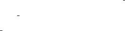
Upon receipt of a HELLO message, a sensor node compares its distance from the sender C of the HELLO message to its sensing range s. A node within a distance s from a coordinator immediately becomes a noncoordinator node and stores the ID of the node that sent the HELLO message in its local cache. A node that is at a distance greater than s from C but within transmission range r becomes eligible to be a coordinator node. This is shown in the Figure 2.1. The shaded region in the figure represents the sensing range of the node C. The outer circle represents the transmission range of the sensor node. Here, we assume that the sensing radius is smaller than the transmission radius. This is often the case for sensors in a sensor node [20].
While SCARE assumes the presence of an appropriate localization mechanism [1–3], exact distance calculations are not necessary. We show later that a moderate error in distance estimation has little effect on the outcome of the self-configuration procedure.
18 SENSOR DEPLOYMENT, SELF-ORGANIZATION, AND LOCALIZATION
r = transmission radius |
s = sensing radius |
C s
Coordinator
r
Eligible to be  noncoordinator
 Eligible to be coordinator
Figure 2.1 Sensing and transmission radii of a node.
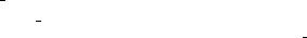
Network Partitioning Problem The basic scheme described above can sometimes result in a partitioning of the network; see Fig. 2.2a. Here, coordinator node F makes node A a non-coordinator. However, coordinator node D can communicate with F only through A. This can potentially result in the partitioning of the network if coordinator (active) node D is unable to reach any other active nodes. As a result, network connectivity cannot be guaranteed in this situation. In Figure 2.2b, G and K are coordinator nodes and B and C are noncoordinator nodes. This situation again results in network partitioning as nodes G and K cannot reach each other.
To prevent such situations, we extend the basic SCARE scheme outlined above, which results in a more effective technique for self-configuration. In the basic scheme, if there is a network partition, a node might never receive a HELLO message. This results in the node waiting eternally for a HELLO message, which results in wastage of energy. Hence, we choose a time-out value Toff after which the nodes that are still undecided about their state can become eligible to become coordinator nodes. The time-out value can be chosen based on the probability threshold discussed in Section 2.2.3. A lower value for the threshold means that the procedure converges quickly and needs a lower Toff value and vice versa.
To prevent the network partitioning that occurs due to the pathological cases shown in Figure 2.2, a node that initially receives a HELLO message from a coordinator node does not become a noncoordinator immediately and go to the sleep state. Instead, it continues to listen for messages from other coordinator nodes and remains in the “eligible to be a
|
|
|
Coordinator |
s = sensing radius |
||
|
|
|
Noncoordinator |
r = transmission radius |
||
|
r |
|
D |
r |
r |
|
|
|
|
|
|||
|
|
|
|
|
||
s |
|
A |
s |
B |
C |
s |
F |
|
G |
K |
|||
|
|
|||||
|
|
|
|
|||
(a) (b)
Figure 2.2 Network partitions in the basic scheme: (a) first scenario and (b) second scenario.
2.2 SCARE |
19 |
noncoordinator” (ETNC) state. A sensor node that is in the ETNC state can become a coordinator node in two cases:
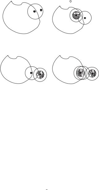
1.If it can connect two neighboring coordinator nodes1 that cannot reach each other in one or two hops. It can deduce this information from the HELLO messages it received earlier. As shown in Figure 2.2a, node A, which is in the ETNC state, receives HELLO messages from node F and node D and decides to become a coordinator; this eliminates the partition.
2.If it can connect two neighboring coordinator nodes that cannot reach each other in one or two hops via a node in the ETNC state. As shown in Figure 2.2b, nodes B and C, that are in the ETNC state, receive HELLO messages from nodes G and K, respectively, and decide to become coordinators as there is no match between the node lists of G and K; this eliminates the partition.
To achieve this, each ETNC node sends a CHECK message. This CHECK message contains the neighbor list of the coordinator node that caused this node to be in the ETNC state. Intuitively, this case is more likely to occur if there are few coordinators in the vicinity and less likely if there are more coordinator neighbors. Any ETNC node that receives this CHECK message replies with a CHECK REPLY message and becomes a coordinator if there is no node common to the neighbor lists of both the nodes. Upon receipt of the CHECK REPLY message, the node that sent the CHECK message also becomes a coordinator. In Figure 2.2b, noncoordinator node B sends a CHECK message and gets a CHECK REPLY message from node C. Both nodes B and C, therefore, become coordinator nodes. This procedure removes the network partition.
If the HELLO message is received from the same partition, and the node lists contained in the HELLO message do not have any common neighbors with the node lists the node received from other HELLO messages, then the node goes from the ETNC state to the “eligible to be coordinator” (ETC) state. This removes partitions if the HELLO messages are from different partitions. If they are from the same partitions, then the node connects the two coordinator nodes.
To prevent oscillations during the selection of coordinators, we enforce the condition that once a node becomes a coordinator, it continues to remain a coordinator until it is unable to provide any service. This strategy is used despite the fact that this coordinator might become redundant later during self-configuration. This penalty is reasonable since it occurs infrequently, especially in contrast to the energy needed to select an optimum number of coordinators. As the density of nodes increases, the fraction of noncoordinator nodes increases, and this leads to more energy savings. Due to its distributed nature, SCARE has a slightly larger number of coordinators than the minimum number necessary for coverage and connectivity. This also happens due to the randomness involved in the distributed selection of coordinator nodes.
After self-configuration, each coordinator periodically broadcasts a HELLO message along with a list of its one-hop neighbors that are coordinators. Noncoordinator nodes listen to these messages. Noncoordinator nodes also maintain a timer to keep track of the coordinator node that made them a noncoordinator. If this timer goes off, a noncoordinator
1 A neighboring node lies within the node’s transmission radius.

20 SENSOR DEPLOYMENT, SELF-ORGANIZATION, AND LOCALIZATION
node assumes that the corresponding coordinator node has failed and goes into an undecided state. This results in noncoordinator nodes becoming eligible to become coordinators.
SCARE can also be applied to mobile sensor networks. A node that has moved to a new location is treated in the same way as the appearance of a new node at that location. It sets itself to the undecided state and listens to the network until either the timer Toff goes off or it receives a HELLO message. Similarly, when a node moves away from one location, this is treated as a node failure by its neighbors. Failure of noncoordinator nodes does not result in any change in the topology. However, the movement of coordinator nodes is detected by the noncoordinator nodes, and this makes them eligible to subsequently become coordinators.
2.2.4 Details of SCARE
A set of control rules governs the state of the sensor node, while a set of defer rules decide when a node should postpone its decision. Timeout rules specify the time after which sensor nodes should make a decision.
A sensor node executing the SCARE procedure can be in one of the following states: coordinator (C), noncoordinator (NC), eligible to be a coordinator (ETC), eligible to be a noncoordinator (ETNC), and undecided (U) (Fig. 2.3). The ETC and ETNC states are temporary and exist only during the Tsetup period explained below. There are seven timeout values in SCARE:
1. Toff Time after which a node that is in the undecided state about its state becomes eligible to be a coordinator and goes into the ETC state.
2.Trand Time for which the sensor node that is in ETC state waits before becoming a coordinator. It then sends a HELLO message along with all its coordinator neighbors that it has identified.
|
|
|
t > Trand |
|
|
|
|
|
|
|||
|
|
|
d > r/2 |
|
C |
Received/Sent |
||||||
|
|
|
|
|
or |
|
CHECK_REPLY |
|||||
|
|
|
|
|
|
|
|
|
|
t > Tsetup |
||
t > Toff |
|
|
DNR Hello |
|||||||||
ETC |
|
|
|
|
|
|
|
|
|
|
||
DNR Hello |
|
|
|
t > |
|
|
|
|
|
|
|
|
|
|
|
T |
coord |
NC |
|||||||
|
|
|
|
|||||||||
|
|
|
|
|
||||||||
|
|
|
|
|
NCN |
|
|
|
|
|
||
t < Toff |
Hello |
|
|
|
|
|
|
|
Awake |
|||
|
|
|
|
|
|
|
|
|
||||
|
|
|
|
|
|
|
|
|
|
|||
t > Toff |
d < r/2 |
|
|
|
|
|
t > Trt |
|||||
|
|
|
|
|
|
t > T |
|
|
||||
U |
t > Trand |
|
|
|
|
|
|
|
setup |
|||
|
|
|
|
Received/Sent |
|
|
||||||
Hello |
|
|
|
|
|
|
|
|||||
|
|
|
|
|
|
CHECK_ |
REPLY |
|||||
d > r/2 |
|
|
|
|
|
|
||||||
t > Toff |
|
|
|
|
|
|
|
|
|
|
|
t > Tsetup |
|
|
|
|
|
|
|
|
|
|
|
DNR |
|
Hello |
|
|
|
|
|
t > Tsetup |
CHECK_REPLY |
|||||
ETNC |
|
|
NC |
|||||||||
d < r/2 |
|
|
|
|
|
|
|
|
Asleep |
|||
|
|
|
DNR |
|||||||||
|
|
|
|
|
|
|
||||||
t > T failure |
|
CHECK_REPLY |
|
|||||||||
|
|
|
|
|
|
|
|
|
|
|||
DNR Hello |
|
|
|
|
|
|
|
|
|
|
||
DNR = Did not receive |
|
|
|
|
|
|
NCN = No common neighbors |
|||||
t = time elapsed |
|
|
|
|
|
|
Trt = Truntime |
|||||
Figure 2.3 State diagram of SCARE.

2.2 SCARE |
21 |
3.Truntime After every Truntime units of time, all noncoordinator nodes wakeup and listen.
4.Tsetup Time interval for which the noncoordinator nodes wake up and listen, after which they go to sleep if they still remain noncoordinators. This is also the period during which beacon messages are sent to synchronize the nodes.
5.Tcoord Time interval during which only the coordinators send HELLO messages. This occurs at the beginning of the Tsetup period.
6.Tnoncoord Time interval during which only the noncoordinators send messages. This is the latter part of the Tsetup period. This period starts immediately after the Tcoord period ends.
7.Tfailure A noncoordinator node waits for time Tfailure for the HELLO messages from the coordinator node that made it the noncoordinator. If no HELLO message is received within this time interval, it decides that the corresponding coordinator node has failed and sets its state to undecided.
Next we describe the type of messages in more detail. There are three types of messages in SCARE:
|
HELLO |
These messages are sent by coordinators. They also contain a list of the one- |
|
hop coordinator neighbors of the sender node. |
|
|
CHECK |
These messages are periodically sent by the noncoordinator nodes. They are |
|
used to remove the potential network partitions. Each CHECK message also contains of |
|
list of coordinator neighbors of the node that made it the noncoordinator. |
|
CHECK REPLY Upon receipt of a CHECK message, noncoordinator node compares |
|
the coordinator neighbor list included in the CHECK message with the neighbor list of |
|
the node that made it a noncoordinator. If there are no common entries in the two lists, |
|
it sends a CHECK REPLY message. Thus, SCARE adopts a conservative strategy in |
|
creating paths in the network and prevent partitions. A noncoordinator node becomes a |
|
coordinator node if two coordinators at the end of the Tcoord period cannot reach each |
|
other within one or two hops. |
Recall that we used r to denote the transmission radius of a node. Similarly, recall that s is the sensing radius of a node. The control rules that decide the state of the sensor node are as follows:
1.A sensor node that generates a random number between 0 and 1, and greater than a threshold, becomes a coordinator.
2.A sensor node that lies at a distance between s and r of a coordinator node becomes eligible to become a coordinator node and goes into the ETC state.
3.A sensor node that lies at a distance at most s from a coordinator node becomes eligible to become a noncoordinator node and goes into the ETNC state.
4.A sensor node that is in ETNC state listens to the HELLO messages sent by the coordinator nodes for the Tcoord period. From this list of coordinator nodes contained in the HELLO messages, if it determines that two coordinator nodes do not have a common neighbor that is a coordinator, this node becomes a coordinator at the end of the Tcoord period. On the other hand, if there are common neighbors in the node lists, then the node stays in the ETNC state.
22SENSOR DEPLOYMENT, SELF-ORGANIZATION, AND LOCALIZATION
5.A sensor node that is in the ETNC state at the end of Tcoord period broadcasts a CHECK message. This message contains a list of the coordinator neighbors of the node that caused it to go to the ETNC state.
6.A sensor node that receives a CHECK message compares the list of neighbors in the CHECK message with its neighbor list. If there is no match between the two lists, it transmits a CHECK REPLY message to the sender of the CHECK message.
7.Upon receipt of a CHECK REPLY to its CHECK message, a sender node that is in the ETNC state becomes a coordinator node. The node that sent the CHECK REPLY also becomes a coordinator.
8.A sensor node that is in the ETNC state and does not satisfy conditions 4 and 5 becomes a noncoordinator node at the end of the setup period.
9.A sensor node that is in the ETC state becomes a coordinator node after the Tcoord period if it does not become a noncoordinator node due to the selection of some other coordinator node.
10.A sensor node with data to send can opt to become a coordinator for as long as it has data to transmit.
The defer rules for SCARE are as follows:
1.If a node becomes eligible to be a coordinator, it listens for Trand period.
2.If a node becomes eligible to be a noncoordinator at the end of the Tcoord period, it listens for time Tnoncoord period.
The timeout rules are as follows:
1.A sensor node at the end of the Trand period broadcasts a HELLO message.
2.A sensor node at the end of the Tsetup period becomes a noncoordinator if it is still eligible to be a noncoordinator.
3.A sensor node at the end of the Tcoord becomes a coordinator if it is still eligible to become a coordinator.
4.A sensor node wakes up and listens to the medium after the timer Truntime expires.
5.After its Toff timer expires, a sensor node becomes eligible to become a coordinator if it is still undecided about its state.
A state diagram for the SCARE algorithm is shown in Figure 2.3. The distance estimate is denoted by d, and we set s = r/2 in this figure. The timeout values in SCARE are application-dependent, and they need to be tuned specific to the application. For example, the Toff value that triggers the state transition from an undecided state to an ETNC state depends on the radio range of the specific sensor used in the sensor network.
Time Relationships The relationships between Toff, Truntime, Tsetup, Tcoord, and Tnoncoord
are as follows:
1.Toff < Tcoord < Tsetup.
2.Tcoord < Tsetup and Tnon−coord < Tsetup.

2.2 SCARE |
23 |
Tcoord 
 Tnoncoord
|
|
|
|
|
T setup |
|
|
|
|
|
|
|
|
|
|
||||
|
|
|
|
|
|
|
|
|
|
|
|
|
|
|
|||||
|
|
|
|
|
|
|
|
|
|
|
|
|
|
|
|
|
|
|
|
|
|
|
|
|
|
|
|
|
|
|
|
|
|
|
|
|
|
|
|
|
|
Ts |
|
Tr |
|
|
|
|
Ts |
|
|
Tr |
|
|
|
|
|
||
|
|
|
|
|
|
|
|
|
|
|
|
|
|||||||
T |
= |
T |
|
T |
|
= |
T |
|
|
|
|
|
|
|
|
|
|||
|
s |
|
r |
|
runtime |
|
|
|
|
|
|
||||||||
|
|
|
setup |
|
|
|
|
|
|
|
|
|
|
|
|||||
Figure 2.4 Illustration of the relationships between the time intervals.
These relationships are illustrated in Figure 2.4.
Figure 2.5 shows the result of applying SCARE to an example sensor network with 100 randomly deployed nodes in a 100-m × 100-m grid. The sensor nodes have a radio range of 25 m. Timeout values of Tfailure of 3 s, Tcoord of 3 s, Tnoncoord of 2 s, Tsetup of 5 s, and Truntime of 95 s are used. SCARE selects 32 nodes as coordinators and the rest are designated as noncoordinators.
Ensuring Network Connectivity We next discuss how SCARE prevents network partitioning. Let S be a set of nodes containing the partial set of coordinators that are connected and the associated nodes in the ETNC state. Each coordinator in set S can reach any other coordinator in set S in a finite number of hops. Let X denote the region enclosing the nodes present in set S. Now consider a node not in set S. Any node not present in S can lead to the following scenarios. We use the notation PA to represent the area within the transmission range of node A.
100
90
80
70
60
50
40
30
20
10
0
0 |
10 |
20 |
30 |
40 |
50 |
60 |
70 |
80 |
90 |
100 |
|
|
|
|
Coordinator |
Noncoordinator |
|
|
|||
Figure 2.5 Result of self-configuration using SCARE.
24 SENSOR DEPLOYMENT, SELF-ORGANIZATION, AND LOCALIZATION
P |
= Node in ETNC state |
A |
|
B |
PA |
A |
QB |
|
A C |
|
B |
X |
|
|
X |
(a) (b)
 = Coordinator
PA
Q B
X A B C
(c)
|
P |
Q |
|
A |
C |
|
|
RB |
X |
A |
B |
|
||
|
C |
D |
(d )
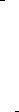
Figure 2.6 Illustration of how network partitioning is prevented in SCARE.
1.Coordinator B outside the region X but within the transmission range of the coordinator A in region X as shown in Figure 2.6a. In this case, both the coordinators can reach each other and the set S = S {B} and the region X expands to include the coordinator B.
2.Coordinator B is outside the transmission range of the coordinator A but is within the transmission range of ETNC node C; see Figure 2.6b. However, as node C listens to the HELLO messages from both coordinator nodes A and B, it becomes a coordinator if there is no other path from A to B by becoming a coordinator. Now this reduces to (case 1) with coordinators C and B within reach of each other. C becomes a coordinator, and the region X expands to include the coordinator B, that is, S = S {B}.
3.Coordinator B is outside the transmission range of coordinator A. However, node C in ETNC state due to node B is within the reach of coordinator A as shown in Figure 2.6c. Node C listens to HELLO messages from A and B, and it becomes a coordinator. Now, A and C are within reach of each other, and this reduces to case 2; hence S = S {C}. By a similar procedure, node B is also included.
4.Coordinator B and coordinator A cannot reach each other as shown in Figure 2.6d. However, nodes C and D that are in ETNC state can reach other. Node C and node D send and receive CHECK and CHECK REPLY messages and become coordinators if there is no other path from node A to B. Once C becomes a coordinator, coordinator C in region X and coordinator D outside region X are within reach of each other. This reduces to case 2 and S = S {D}. Region X expands to include node B and node D.
5.A node F that is outside the reach of either a coordinator or a node in ETNC state in region X . In this case, as the region X expands to include more nodes, node F falls into one of the above categories and as a consequence becomes connected with the nodes present in region X .
We have therefore shown that network partitioning can never arise during self-configuration.
2.2 SCARE |
25 |
Message Complexity The total number of control messages, referred to as message complexity in SCARE, can be determined as follows: Suppose N is the total number of nodes in the network. Let Nc be the number of coordinator nodes selected. The number of noncoordinator nodes in the network is then simply N − Nc. Each coordinator node sends a HELLO message and each noncoordinator node sends a CHECK message. Let be the average number of coordinator neighbors of a noncoordinator node. A noncoordinator node sends a CHECK REPLY message in response to a CHECK message if and only if there is no match between the coordinator neighbor lists of the noncoordinator nodes. In Span, each noncoordinator node sends one message and each coordinator node sends two messages. Therefore, the number of messages sent in each Tperiod interval is N + Nc.
Consider two noncoordinator nodes A and B. For every node in the coordinator neighbor list of A, let α be the probability that this node is present in the coordinator neighbor list of node B. The probability that there are is no match is then (1 − α) . Thus the expected number of CHECK REPLY messages is (1 − α) (N − Nc). The total expected number of control messages sent in SCARE is therefore (1 − α) (N − Nc) + Nc + (N − Nc) ≈ N for sufficiently large in dense sensor networks. This is clearly less than the N + Nc messages needed in Span. The size of each message in SCARE is almost equal to the size of each message in Span since the almost same information is contained in both sets of messages.
2.2.5 Optimal Centralized Algorithm
In this section, we develop a provably optimal centralized algorithm that selects a smallest number of nodes to maximize coverage yet maintains network connectivity. This optimal algorithm is compared to SCARE in order to evaluate the effectiveness of the distributed algorithm.
We model the sensor network as a graph G, and use this model to develop an algorithm MAXCOVSPAN that generates a spanning subgraph of G. In addition, G provides the maximum coverage among all spanning subgraps of G, where the nodes in the spanning subgraph correspond to the active sensor nodes in the network. The results provided by the centralized procedure MAXCOVSPAN can then be compared with the results obtained using the distributed SCARE procedure.
Recall that SCARE selects nodes as coordinators on the basis of a distance metric. MAXCOVSPAN also uses the distance between nodes to include nodes in a spanning subgraph such that the coverage is maximized.
Problem Statement Find a spanning subgraph of G that provides the maximum coverage. The vertices in G correspond to the sensor nodes. If two nodes are within radio range of each other, an edge is included in G between the corresponding vertices. The weight of this edge denotes the distance between the two sensor nodes. The algorithm is described in terms of the following rules that are applied to G.
Initialization
Rule 0: Color all vertices white.
Rule 1: Start with an arbitrary node. Call this node Current and color it black.
26 SENSOR DEPLOYMENT, SELF-ORGANIZATION, AND LOCALIZATION
Selection
Rule 2: Pick an adjacent vertex that is connected by an edge to the Current vertex of maximum weight and color this node black. Color all other neighbors of the Current node gray. Call the vertex that has most recently been colored black as Current.
Rule 3: If the vertex belonging to the longest edge is already colored black, follow rule 4; otherwise repeat rule 2.
Rule 4: If there are still white vertices, pick a gray vertex that has most white neighbor vertices and call it Current.
Termination
Rule 5: Repeat rules 2, 3, and 4 until all the vertices are colored either black or gray.
Theorem 2.2.1 The algorithm MAXCOVSPAN runs in O(n2) time for a graph with n vertices.
PROOF At each time instant, one vertex is colored either black or gray. There are n vertices in the graph. However, we need to check for the remaining gray nodes that have white nodes as their neighbors. This takes O(n) time as we might have to check all the n nodes in the worst case. Hence, it takes a total of O(n2) time to complete the algorithm. 
Theorem 2.2.2 MAXCOVSPAN always generates a spanning subgraph.
PROOF It suffices to show that at the end of the algorithm, each node is colored either gray or black. This can be shown as follows. According to rule 4, if a gray node has white vertices as neighbors, then it is colored black and all its neighbors except the neighboring vertex belonging to the longest edge are colored gray. A black node has all its neighbors colored black or gray according to rule 2. This completes the proof of the theorem. 
Theorem 2.2.3 The spanning subgraph G generated by MAXCOVSPAN provides the
highest coverage among all spanning subgraphs of G that have the same number of nodes as G .
PROOF In order to avoid case-by-case analysis, we prove this theorem using mathematical induction. Suppose G = (V , E) is the graph corresponding to the sensor network. Let Pi = (Vi , Ei ) denote the partial (incomplete) spanning subgraph of size i generated by MAXCOVSPAN. Let Cov(Pi ) denote the coverage obtained with Pi . Consider the base case P1 = (v1, φ), where v1 is any node selected at random. Cov(P1) is the maximum as all nodes have the same sensing range, and the coverage provided by any node is the same. Next we assume that that the coverage of Pn is the maximum among all partial spanning subgraphs of size n. The coverage provided by a partial connected spanning subgraph of
size n + 1 is given by Cov(Pn+1) = Cov(Pn ) |
|
Cov(v2) where v2 is the node added to |
||
the partial spanning subgraph of size n. For |
Cov(P |
) to be maximum, v needs to have |
||
|
|
n+1 |
2 |
|
minimum overlap with Pn . This is ensured by MAXCOVSPAN. The algorithm selects the node that is farthest from the partial spanning subgraph, and this results in the coverage of the new selected node to have minimum overlap with the partial spanning subgraph of size

2.2 SCARE |
27 |
n. From this observation, it follows that Cov(Pn+1) is maximum. Hence by the principle of mathematical induction, we have shown that MAXCOVSPAN generates a connected spanning subgraph that provides maximum coverage. 
Coverage Comparisons Figure 2.7 shows the variation of coverage with the total number of nodes for three scenarios: all nodes awake, MAXCOVSPAN, and SCARE. We assume that the nodes are placed randomly on a 100-m × 100-m grid. We assume a sensing range of 12.5 m and a transmission range of 25 m. We vary the number of nodes from 50 to 300, and the results are averaged over 100 runs. The results show that the distributed SCARE procedure performs nearly as well as the centralized MAXCOVSPAN procedure, and for a large rnumber of deployed nodes, both these methods perform nearly as well as the scheme of keeping all nodes awake.
2.2.6 Performance Evaluation
To better understand the performance issues in SCARE, we use simulations to determine the effectiveness of SCARE in terms of coverage, connectedness, and network lifetime. We compare SCARE to Span in the simulations. Finally, we examine the impact of distance estimation errors on the effectiveness of SCARE.
Each sensor node is assumed to have a radio range of 25 m. The bandwidth of the radio is assumed to be 20 kbps. The sensor characteristics are given in Table 2.1 [21].
Simulation Methodology We have developed a simulator in Java to evaluate the performance of SCARE. Our simulator uses geographic forwarding as the routing layer and
|
10000 |
|
|
|
|
|
|
9800 |
|
|
|
|
|
|
9600 |
|
|
|
|
|
|
9400 |
|
|
|
|
|
) |
9200 |
|
|
|
|
|
2 |
|
|
|
|
|
|
(m |
|
|
|
|
|
|
Coverage |
9000 |
|
|
|
|
|
8800 |
|
|
|
|
|
|
|
8600 |
|
|
|
|
|
|
8400 |
|
|
All nodes awake |
|
|
|
|
|
SCARE |
|
|
|
|
|
|
|
Spanning subgraph algorithm |
|
|
|
8200 |
|
|
|
|
|
|
8000 |
100 |
150 |
200 |
250 |
300 |
|
50 |
Total number of nodes
Figure 2.7 Coverage versus number of nodes.
28 SENSOR DEPLOYMENT, SELF-ORGANIZATION, AND LOCALIZATION
Table 2.1 Radio Characteristics [21].
Radio Mode |
Power Consumption (mW) |
|
|
Transmit (Tx ) |
14.88 |
Receive (Rx ) |
12.50 |
Idle |
12.36 |
Sleep |
0.016 |
|
|
IEEE 802.11 [22] as the MAC layer. Each sensor node that receives a packet forwards it to the neighbor coordinator node that is closest to the destination. If no neighboring coordinator node is closer to the destination than the node itself, the packet cannot be forwarded and it is dropped. SCARE runs on top of IEEE 802.11 MAC and below the routing layer to help coordinate the forwarding of packets from source to destination.
We use a grid size of 100 m × 100 m, and sensor nodes with radios having a nominal radio range of 25 m and a bandwidth of 20 kbps. Initially, nodes are randomly deployed in the grid with the only condition that the nodes form a connected network. We simulate different node densities by increasing the number of nodes and keeping the grid size constant. To study the effect of increase in the number of nodes on SCARE, we simulate 50, 100, 150, 200, 250, and 300 nodes in our simulations. The results presented in this section are averaged over 100 simulation runs.
In the remainder of this section, we compare SCARE with Span and show that SCARE selects a smaller number of coordinators compared to Span and thus provides significant energy savings. To study the effect of SCARE coordinator selection on packet loss rate, we used a constant bit rate (CBR) traffic. However, to more closely understand the effectiveness of SCARE, we separate the nodes that generate traffic from the nodes that execute SCARE and participate in multihop forwarding of packets. Sources and destinations of traffic are placed outside the simulated region, and these nodes do not execute the SCARE procedure. A total of 10 source nodes and 10 destination nodes are used in our simulations. Each source node selects a random destination from the 10 destination nodes and sends a CBR traffic of 10 kbps to it.
To study the effect of mobility on SCARE, we use a random way-point model [23]. In this model, each node randomly selects a destination location in the sensor field and starts moving toward it with a velocity randomly chosen from a uniform distribution. Once it reaches the destination, it waits for a certain predetermined pause time, before it starts moving again. The pause time determines the degree of mobility in this model. We simulated five different pause times of 0, 100, 200, 500, and 1000 s and a velocity range of 0 to 10 m/s. A pause time of 1000 s corresponds to the stationary sensor network while a pause time of 0 s corresponds to high mobility. We used Tfailure = 3 s, Tcoord = 3 s, Tnoncoord = 2 s, Tsetup = 5 s, and Truntime = 95 s in our simulations.
Although SCARE relies on a localization scheme, we do not simulate it in our simulator for simplicity. Instead, we make use of the geographic locations of sensor nodes provided by our simulator to aid SCARE in deciding the state of each sensor node. However, since the message overhead due to SCARE is negligible, only one message per node, we believe that this does not affect the results significantly.
Simulation Results In this subsubsection, we first evaluate the coverage provided by SCARE. We define coverage as the total sensing area spanned by all the coordinator nodes.
2.2 SCARE |
29 |
|
10000 |
|
|
|
|
|
|
9800 |
|
|
|
|
|
|
9600 |
|
|
|
|
|
|
9400 |
|
|
|
|
|
Coverage |
9200 |
|
|
|
|
|
9000 |
|
|
|
|
|
|
8800 |
|
|
|
|
|
|
|
|
|
|
|
|
|
|
8600 |
|
|
|
|
|
|
8400 |
|
|
|
|
|
|
|
|
|
|
|
All nodes |
|
8200 |
|
|
|
|
SCARE |
|
8000 |
|
|
|
|
|
|
50 |
100 |
150 |
200 |
250 |
300 |
Number of nodes
Figure 2.8 Coverage obtained with SCARE compared to the case when all nodes are awake.
We assume that noncoordinator nodes turn off their sensors. Although SCARE does not provide complete coverage due to the random deployment gaps in the sensing range of the coordinators, its coverage is very close to the maximum coverage. Yet, SCARE selects only a few nodes as coordinators to provide this coverage, thus achieving considerable energy savings. Therefore, SCARE efficiently trades off minimum loss in coverage with a tremendous gain in energy savings.
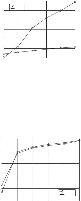
In Figure 2.8, we show the coverage versus the number of deployed nodes for SCARE. Recall that coverage is measured by the total sensing area spanned by all the coordinator nodes. We also show the coverage when SCARE is not run and all nodes are kept awake. As expected, the coverage obtained with SCARE is slightly less than the coverage obtained if all nodes have their sensors and radios turned on. However, the coverage produced by SCARE becomes comparable to the best-case coverage as the number of nodes increases. In these simulations, the grid size is kept constant, hence an increase in the number of nodes represents an increase in the node density.
We next compare the number of coordinators selected in Span with the corresponding number for SCARE. As shown in Figure 2.9, the number of coordinators selected by SCARE is much less than in Span. (For 50 nodes, Span selects fewer coordinators, but the coverage is too low.) SCARE selects a smaller number of coordinators yet provides nearly the same coverage.
Figure 2.10 shows the coverage obtained by using SCARE and Span. SCARE tends to provide better coverage than Span for a range of values for the number of nodes below 100. Both provide similar coverage as the number of nodes increases beyond a threshold.
Figure 2.11 shows the fraction of nodes selected as coordinators with an increase in the number of nodes. SCARE selects a small fraction of nodes as coordinators with increase in node density. Hence, compared to Span, more energy savings are obtained with SCARE for dense sensor networks.
Figure 2.12 compares the number of coordinators selected by SCARE compared to the ideal number of coordinators needed for the square tiling configuration discussed in
30 SENSOR DEPLOYMENT, SELF-ORGANIZATION, AND LOCALIZATION
|
140 |
|
|
|
|
|
|
|
Span |
|
|
|
|
|
120 |
SCARE |
|
|
|
|
elected |
|
|
|
|
|
|
100 |
|
|
|
|
|
|
of coordinators |
|
|
|
|
|
|
80 |
|
|
|
|
|
|
60 |
|
|
|
|
|
|
Number |
|
|
|
|
|
|
40 |
|
|
|
|
|
|
|
|
|
|
|
|
|
|
20 |
|
|
|
|
|
|
50 |
100 |
150 |
200 |
250 |
300 |
Number of nodes
Figure 2.9 Number of coordinators selected with an increase in nodes.
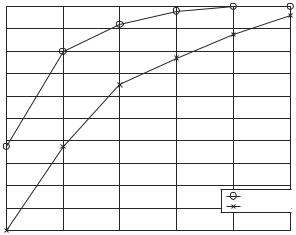
Section 2.2.5. SCARE selects almost the same number of coordinators as in the ideal case. This behavior is different from the behavior of SCARE in Figure 2.9 as here the nodes are placed in a regular fashion and not randomly deployed. Random deployment results in SCARE selecting more nodes as coordinators to cover the entire grid and still maintain connectivity. Any self-configuration algorithm should have minimal control message overhead. In Figure 2.13, we compare the number of control messages used by SCARE and Span for the self-configuration. SCARE uses a smaller number of control messages compared to Span because it takes advantage of the random initialization of the nodes. This leads to a partial configuration of the network; hence SCARE uses fewer number of control messages to achieve self-configuration.
|
10000 |
|
|
|
|
|
|
9500 |
|
|
|
|
|
Coverage |
9000 |
|
|
|
|
|
8500 |
|
|
|
|
|
|
|
|
|
|
|
|
|
|
8000 |
|
|
|
|
|
|
|
|
|
|
Span |
|
|
|
|
|
|
SCARE |
|
|
7500 |
|
|
|
|
|
|
50 |
100 |
150 |
200 |
250 |
300 |
Number of nodes
Figure 2.10 Coverage versus number of nodes for SCARE and Span.

2.2 SCARE |
31 |
|
60 |
|
|
|
|
SCARE |
|
|
|
|
|
|
|
as coordinators |
55 |
|
|
|
|
Span |
50 |
|
|
|
|
|
|
45 |
|
|
|
|
|
|
40 |
|
|
|
|
|
|
elected |
|
|
|
|
|
|
35 |
|
|
|
|
|
|
|
|
|
|
|
|
|
of nodes |
30 |
|
|
|
|
|
25 |
|
|
|
|
|
|
Fraction |
20 |
|
|
|
|
|
15 |
|
|
|
|
|
|
|
|
|
|
|
|
|
|
10 |
100 |
150 |
200 |
250 |
300 |
|
50 |
Number of nodes
Figure 2.11 Fraction of nodes selected as coordinators in SCARE and Span.
Figure 2.14 shows the effects of mobility on packet loss rate for both Span and SCARE. Nodes follow the random way-point model described in the previous subsubsection. Packet loss rate is calculated as the ratio of the number of lost packets to the number of packets actually sent. We note that the packet loss rates for both these methods are comparable.
Figure 2.15 shows the fraction of surviving nodes as a function of simulation time for both SCARE and Span. SCARE uses fewer control messages and consumes less energy for self-configuration and reconfiguration of the network. The number of surviving nodes falls below 80% at 765 for SCARE compared to 700 for Span.
|
50 |
|
|
|
|
|
|
|
|
|
|
Ideal |
|
|
|
|
|
|
SCARE |
|
coordinators |
45 |
|
|
|
|
|
40 |
|
|
|
|
|
|
|
|
|
|
|
|
|
of selected |
35 |
|
|
|
|
|
30 |
|
|
|
|
|
|
Number |
|
|
|
|
|
|
25 |
|
|
|
|
|
|
|
|
|
|
|
|
|
|
20 |
|
|
|
|
|
|
50 |
100 |
150 |
200 |
250 |
300 |
Number of nodes
Figure 2.12 Coordinators selected in SCARE versus an ideal number of coordinators selected based on square tiling.

32 SENSOR DEPLOYMENT, SELF-ORGANIZATION, AND LOCALIZATION
|
1400 |
|
|
|
|
|
|
|
|
|
|
|
1200 |
|
Span |
|
|
|
|
|
|
|
|
|
|
SCARE |
|
|
|
|
|
|
|
||
|
|
|
|
|
|
|
|
|
|
||
messages |
1000 |
|
|
|
|
|
|
|
|
|
|
|
|
|
|
|
|
|
|
|
|
|
|
of control |
800 |
|
|
|
|
|
|
|
|
|
|
600 |
|
|
|
|
|
|
|
|
|
|
|
number |
|
|
|
|
|
|
|
|
|
|
|
400 |
|
|
|
|
|
|
|
|
|
|
|
Total |
|
|
|
|
|
|
|
|
|
|
|
|
|
|
|
|
|
|
|
|
|
|
|
|
200 |
|
|
|
|
|
|
|
|
|
|
|
0 |
|
|
|
|
|
|
|
|
|
|
|
0 |
100 |
200 |
300 |
400 |
500 |
600 |
700 |
800 |
900 |
1000 |
Simulation time (s)
Figure 2.13 Number of control messages used for self-configuration.
Effect of Location Estimation Error on Results We next investigate how errors in distance estimation affect the performance of SCARE. Since nodes use distance estimation only to determine their eligibility to go to the sleep state, we do not expect SCARE to be significantly affected because of moderate errors in distance estimates.
To measure this feature of SCARE quantitatively, we ran simulations by introducing artificial errors in distance estimation. We modeled such errors by shifting the location of each node by a random amount in the range [x ± e, y ± e], where e is either 10 or 20% of the radio range of a node and [x, y] is the location of a sensor node. Nodes use these
|
16 x 10−3 |
|
|
|
|
|
|
|
|
|
|
|
|
|
|
|
|
|
SCARE |
|
|
|
14 |
|
|
|
|
|
|
Span |
|
|
|
|
|
|
|
|
|
|
|
|
|
|
12 |
|
|
|
|
|
|
|
|
|
rate |
10 |
|
|
|
|
|
|
|
|
|
loss |
|
|
|
|
|
|
|
|
|
|
|
|
|
|
|
|
|
|
|
|
|
Packet |
8 |
|
|
|
|
|
|
|
|
|
|
|
|
|
|
|
|
|
|
|
|
|
6 |
|
|
|
|
|
|
|
|
|
|
4 |
|
|
|
|
|
|
|
|
|
|
2 |
200 |
300 |
400 |
500 |
600 |
700 |
800 |
900 |
1000 |
|
100 |
Pause time (s)
Figure 2.14 Packet loss rate as a function of pause time.

|
|
|
|
|
|
|
2.2 |
SCARE |
33 |
|
|
|
|
|
|
SCARE |
|
|
|
|
1 |
|
|
|
|
Span |
|
|
|
|
|
|
|
|
|
|
|
|
|
nodes |
0.8 |
|
|
|
|
|
|
|
|
|
|
|
|
|
|
|
|
|
|
of surviving |
0.6 |
|
|
|
|
|
|
|
|
|
|
|
|
|
|
|
|
|
|
Fraction |
0.4 |
|
|
|
|
|
|
|
|
|
|
|
|
|
|
|
|
|
|
|
0.2 |
|
|
|
|
|
|
|
|
|
0 |
|
|
|
|
|
|
|
|
|
0 |
200 |
400 |
600 |
800 |
1000 |
1200 |
|
|
Simulation time (s)
Figure 2.15 Fraction of nodes remaining with time for Span and SCARE.
artificial locations rather than their real location to estimate the distance between them and a coordinator node. We refer to this scheme as either SCARE-10 or SCARE-20.
Figure 2.16 shows the results of these simulations. The simulations using SCARE-10 and SCARE-20 are based on incorrect estimation of the distance from the coordinators by the nodes. Consequently, the number of coordinators is different from the case when there is no error. However, the increase in the number of coordinators is negligible, while the decrease in coverage is found to be minimal. In the case of SCARE-10, the increase is only 3% for a small number of nodes and negligible (<0.2%) for a large number of nodes.
|
50 |
|
|
|
|
|
|
48 |
|
|
|
|
|
elected |
46 |
|
|
|
|
|
44 |
|
|
|
|
|
|
|
|
|
|
|
|
|
coordinators |
42 |
|
|
|
|
|
40 |
|
|
|
|
|
|
38 |
|
|
|
|
|
|
of |
|
|
|
|
|
|
|
|
|
|
|
|
|
Number |
36 |
|
|
|
|
|
34 |
|
|
|
|
|
|
|
|
|
|
SCARE |
|
|
|
|
|
|
|
|
|
|
32 |
|
|
|
SCARE10 |
|
|
|
|
|
SCARE20 |
|
|
|
|
|
|
|
|
|
|
30 |
|
|
|
|
|
|
50 |
100 |
150 |
200 |
250 |
300 |
Number of nodes
Figure 2.16 Effect of error in distance estimation on SCARE.
34 SENSOR DEPLOYMENT, SELF-ORGANIZATION, AND LOCALIZATION
|
350 |
|
|
|
|
|
|
|
|
300 |
|
|
|
|
|
N = 300 |
|
|
|
|
|
|
|
N = 400 |
|
|
|
|
|
|
|
|
|
|
|
of coordinators |
|
|
|
|
|
|
N = 500 |
|
250 |
|
|
|
|
|
|
|
|
200 |
|
|
|
|
|
|
|
|
150 |
|
|
|
|
|
|
|
|
Number |
|
|
|
|
|
|
|
|
100 |
|
|
|
|
|
|
|
|
|
50 |
|
|
|
|
|
|
|
|
0 |
0.2 |
0.3 |
0.4 |
0.5 |
0.6 |
0.7 |
0.8 |
|
0.1 |
Ratio of sensing to transmission radius
Figure 2.17 Number of coordinators selected versus s/r .
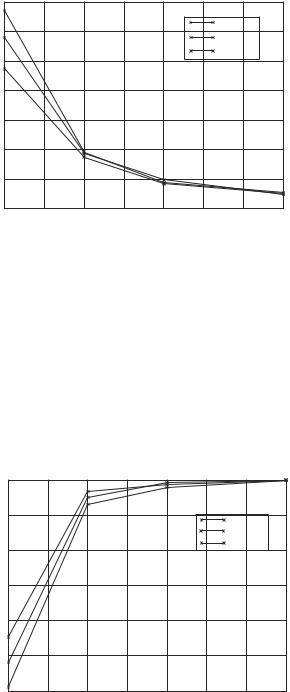
The decrease in coverage was found to be at most 0.7%. As can be seen from the graph in Figure 2.16, the results are similar for the SCARE-20 case.
In all the simulation results shown above, the sensing radius has been taken to be one-half of the transmission radius. We now examine the effect of varying the sensing radius (s) as a fraction of the transmission radius (r ) of a node. Figure 2.17 shows that the number of coordinators selected by SCARE as the ratio of sensing radius to the transmission radius is varied. The number of coordinators selected drops rapidly as the ratio increases. As expected, the coverage increases with an increase in s/r ; see Figure 2.18. At the s/r value of 0.3, we obtain almost 93% coverage with only 25% nodes selected as coordinators.
|
10000 |
|
|
|
|
|
|
|
|
9000 |
|
|
|
|
|
N = 300 |
|
|
|
|
|
|
|
|
|
|
|
|
|
|
|
|
|
N = 400 |
|
|
8000 |
|
|
|
|
|
N = 500 |
|
|
|
|
|
|
|
|
|
|
Coverage |
7000 |
|
|
|
|
|
|
|
|
|
|
|
|
|
|
|
|
|
6000 |
|
|
|
|
|
|
|
|
5000 |
|
|
|
|
|
|
|
|
4000 |
0.2 |
0.3 |
0.4 |
0.5 |
0.6 |
0.7 |
0.8 |
|
0.1 |
Ratio of sensing to transmission radius
Figure 2.18 Coverage obtained versus s/r .