

Fundamentals Of Wireless Communication
.pdf18
Figure 2.6 Illustration of a direct path and a reflected path off a ground plane.
The wireless channel
Transmit antenna |
|
|
|
|
r1 |
|
|
|
|
|
|
hs |
r2 |
Receive antenna |
|
|
|||
|
Ground plane |
|
hr |
|
|
||
|
|
|
|
|
r |
|
|
plane (i.e., height), a very surprising thing happens. In particular, the difference between the direct path length and the reflected path length goes to zero as r−1 with increasing r (Exercise 2.5). When r is large enough, this difference between the path lengths becomes small relative to the wavelength c/f. Since the sign of the electric field is reversed on the reflected path5, these two waves start to cancel each other out. The electric wave at the receiver is then attenuated as r−2, and the received power decreases as r−4. This situation is particularly important in rural areas where base-stations tend to be placed on roads.
2.1.6 Power decay with distance and shadowing
The previous example with reflection from a ground plane suggests that the received power can decrease with distance faster than r−2 in the presence of disturbances to free space. In practice, there are several obstacles between the transmitter and the receiver and, further, the obstacles might also absorb some power while scattering the rest. Thus, one expects the power decay to be considerably faster than r−2. Indeed, empirical evidence from experimental field studies suggests that while power decay near the transmitter is like r−2, at large distances the power can even decay exponentially with distance.
The ray tracing approach used so far provides a high degree of numerical accuracy in determining the electric field at the receiver, but requires a precise physical model including the location of the obstacles. But here, we are only looking for the order of decay of power with distance and can consider an alternative approach. So we look for a model of the physical environment with the fewest parameters but one that still provides useful global information about the field properties. A simple probabilistic model with two parameters of the physical environment, the density of the obstacles and the fraction of energy each object absorbs, is developed in Exercise 2.6. With each obstacle
5This is clearly true if the electric field is parallel to the ground plane. It turns out that this is also true for arbitrary orientations of the electric field, as long as the ground is not a perfect conductor and the angle of incidence is small enough. The underlying electromagnetics is analyzed in Chapter 2 of Jakes [62].
19 2.1 Physical modeling for wireless channels
absorbing the same fraction of the energy impinging on it, the model allows us to show that the power decays exponentially in distance at a rate that is proportional to the density of the obstacles.
With a limit on the transmit power (either at the base-station or at the mobile), the largest distance between the base-station and a mobile at which communication can reliably take place is called the coverage of the cell. For reliable communication, a minimal received power level has to be met and thus the fast decay of power with distance constrains cell coverage. On the other hand, rapid signal attenuation with distance is also helpful; it reduces the interference between adjacent cells. As cellular systems become more popular, however, the major determinant of cell size is the number of mobiles in the cell. In engineering jargon, the cell is said to be capacity limited instead of coverage limited. The size of cells has been steadily decreasing, and one talks of micro cells and pico cells as a response to this effect. With capacity limited cells, the inter-cell interference may be intolerably high. To alleviate the inter-cell interference, neighboring cells use different parts of the frequency spectrum, and frequency is reused at cells that are far enough. Rapid signal attenuation with distance allows frequencies to be reused at closer distances.
The density of obstacles between the transmit and receive antennas depends very much on the physical environment. For example, outdoor plains have very little by way of obstacles while indoor environments pose many obstacles. This randomness in the environment is captured by modeling the density of obstacles and their absorption behavior as random numbers; the overall phenomenon is called shadowing.6 The effect of shadow fading differs from multipath fading in an important way. The duration of a shadow fade lasts for multiple seconds or minutes, and hence occurs at a much slower time-scale compared to multipath fading.
2.1.7 Moving antenna, multiple reflectors
Dealing with multiple reflectors, using the technique of ray tracing, is in principle simply a matter of modeling the received waveform as the sum of the responses from the different paths rather than just two paths. We have seen enough examples, however, to understand that finding the magnitudes and phases of these responses is no simple task. Even for the very simple large wall example in Figure 2.2, the reflected field calculated in (2.6) is valid only at distances from the wall that are small relative to the dimensions of the wall. At very large distances, the total power reflected from the wall is proportional to both d−2 and to the area of the cross section of the wall. The power reaching the receiver is proportional to d − r t−2. Thus, the power attenuation from transmitter to receiver (for the large distance case) is proportional to d d − r t−2 rather
6 This is called shadowing because it is similar to the effect of clouds partly blocking sunlight.

20 The wireless channel
than to 2d − r t−2. This shows that ray tracing must be used with some caution. Fortunately, however, linearity still holds in these more complex cases.
Another type of reflection is known as scattering and can occur in the atmosphere or in reflections from very rough objects. Here there are a very large number of individual paths, and the received waveform is better modeled as an integral over paths with infinitesimally small differences in their lengths, rather than as a sum.
Knowing how to find the amplitude of the reflected field from each type of reflector is helpful in determining the coverage of a base-station (although ultimately experimentation is necessary). This is an important topic if our objective is trying to determine where to place base-stations. Studying this in more depth, however, would take us afield and too far into electromagnetic theory. In addition, we are primarily interested in questions of modulation, detection, multiple access, and network protocols rather than location of base-stations. Thus, we turn our attention to understanding the nature of the aggregate received waveform, given a representation for each reflected wave. This leads to modeling the input/output behavior of a channel rather than the detailed response on each path.
2.2 Input/output model of the wireless channel
We derive an input/output model in this section. We first show that the multipath effects can be modeled as a linear time-varying system. We then obtain a baseband representation of this model. The continuous-time channel is then sampled to obtain a discrete-time model. Finally we incorporate additive noise.
2.2.1 The wireless channel as a linear time-varying system
In the previous section we focused on the response to the sinusoidal input t = cos 2ft. The received signal can be written as i aif t t − if t, where aif t and if t are respectively the overall attenuation and propagation delay at time t from the transmitter to the receiver on path i. The overall attenuation is simply the product of the attenuation factors due to the antenna pattern of the transmitter and the receiver, the nature of the reflector, as well as a factor that is a function of the distance from the transmitting antenna to the reflector and from the reflector to the receive antenna. We have described the channel effect at a particular frequency f. If we further assume that the aif t and the if t do not depend on the frequency f, then we can use the principle of superposition to generalize the above input/output relation to an arbitrary input x t with non-zero bandwidth:
y t = ait x t − it (2.14)
i
21 |
2.2 Input/output model of the wireless channel |
In practice the attenuations and the propagation delays are usually slowly varying functions of frequency. These variations follow from the time-varying path lengths and also from frequency-dependent antenna gains. However, we are primarily interested in transmitting over bands that are narrow relative to the carrier frequency, and over such ranges we can omit this frequency dependence. It should however be noted that although the individual attenuations and delays are assumed to be independent of the frequency, the overall channel response can still vary with frequency due to the fact that different paths have different delays.
For the example of a perfectly reflecting wall in Figure 2.4, then,
a |
t |
|
|
|
|
|
|
a |
t |
|
|
|
|
|
|
|
(2.15) |
= r0 + vt |
|
|
= |
2d − r0 − vt |
|
|
|||||||||||
1 |
|
|
1 |
|
2 |
|
|
2 |
|
|
|||||||
|
t |
= |
|
r0 + vt |
− |
|
|
t |
= |
|
2d − r0 |
− vt |
− |
|
(2.16) |
||
c |
2f |
c |
|
2f |
|||||||||||||
1 |
|
|
|
2 |
|
|
|
|
|
||||||||
where the first expression is for the direct path and the second for the reflected path. The term j here is to account for possible phase changes at the transmitter, reflector, and receiver. For the example here, there is a phase reversal at the reflector so we take 1 = 0 and 2 = .
Since the channel (2.14) is linear, it can be described by the response h t at time t to an impulse transmitted at time t − . In terms of h t, the input/output relationship is given by
|
|
y t = − h t x t − d |
(2.17) |
Comparing (2.17) and (2.14), we see that the impulse response for the fading multipath channel is
h t = ait − it (2.18)
i
This expression is really quite nice. It says that the effect of mobile users, arbitrarily moving reflectors and absorbers, and all of the complexities of solving Maxwell’s equations, finally reduce to an input/output relation between transmit and receive antennas which is simply represented as the impulse response of a linear time-varying channel filter.
The effect of the Doppler shift is not immediately evident in this representation. From (2.16) for the single reflecting wall example, i t = vi/c where vi is the velocity with which the ith path length is increasing. Thus, the Doppler shift on the ith path is −fi t.
In the special case when the transmitter, receiver and the environment are all stationary, the attenuations ait and propagation delays it do not
22 |
The wireless channel |
depend on time t, and we have the usual linear time-invariant channel with an impulse response
h = ai − i (2.19)
i
For the time-varying impulse response h t , we can define a time-varying frequency response
|
|
|
|
|
H f t = − h t e−j2 f d = |
ai t e−j2 f i t |
(2.20) |
||
i |
In the special case when the channel is time-invariant, this reduces to the usual frequency response. One way of interpreting H f t is to think of the system as a slowly varying function of t with a frequency response H f t at each fixed time t. Corresponding, h t can be thought of as the impulse response of the system at a fixed time t. This is a legitimate and useful way of thinking about many multipath fading channels, as the time-scale at which the channel varies is typically much longer than the delay spread (i.e., the amount of memory) of the impulse response at a fixed time. In the reflecting wall example in Section 2.1.4, the time taken for the channel to change significantly is of the order of milliseconds while the delay spread is of the order of microseconds. Fading channels which have this characteristic are sometimes called underspread channels.
2.2.2 Baseband equivalent model
In typical wireless applications, |
communication occurs in a passband |
fc − W/2 fc + W/2 of bandwidth |
W around a center frequency fc, the |
spectrum having been specified by regulatory authorities. However, most of the processing, such as coding/decoding, modulation/demodulation, synchronization, etc., is actually done at the baseband. At the transmitter, the last stage of the operation is to “up-convert” the signal to the carrier frequency and transmit it via the antenna. Similarly, the first step at the receiver is to “down-convert” the RF (radio-frequency) signal to the baseband before further processing. Therefore from a communication system design point of view, it is most useful to have a baseband equivalent representation of the system. We first start with defining the baseband equivalent representation of signals.
Consider a real signal s t with Fourier transform S f , band-limited in
fc − W/2 fc + W/2 with W < 2fc. Define its complex baseband equivalent
sb t as the signal having Fourier transform: |
|
|
||||||
|
|
|
√ |
|
S f |
+ fc |
f + fc > 0 |
|
S |
f |
= |
|
2 |
(2.21) |
|||
b |
|
0 |
|
f + fc ≤ 0 |
|
|||
23
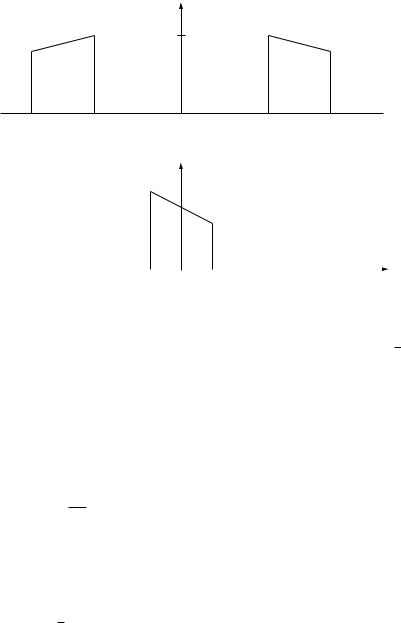
Figure 2.7 Illustration of the relationship between a passband spectrum S(f ) and its baseband equivalent Sb(f ).
2.2 Input/output model of the wireless channel
S( f )
1
 f
f
–fc – |
W |
– fc + |
W |
|
|
|
fc – W |
fc + |
W |
|
2 |
|
2 |
2 |
|
2 |
|||
|
|
|
|
|
Sb ( f ) |
|
|
||
|
|
|
|
|
√ |
|
|
|
|
|
|
|
|
|
2 |
|
|
||
|
|
|
|
|
|
|
|||
|
|
f |
|
|
|
– W |
W |
|
2 |
2 |
|
Since s t is real, its Fourier transform satisfies S f = S −f , which means
√
that sbt contains exactly the same information as s t. The factor of 2 is quite arbitrary but chosen to normalize the energies of sbt and s t to be the same. Note that sbt is band-limited in −W/2 W/2 . See Figure 2.7.
To reconstruct s t from sbt, we observe that |
|
|
|
|
||||||||||||
|
|
|
√ |
|
S f = Sbf − fc + Sb −f − fc |
|
|
|
||||||||
|
|
|
|
2 |
|
|
(2.22) |
|||||||||
Taking inverse Fourier transforms, we get |
|
|
|
|
|
|
|
|
||||||||
1 |
sbte |
j2 fct |
+ sb te− |
j2 fct |
= |
√ |
|
|
sbte |
j2 fct |
|
|
||||
|
|
|||||||||||||||
s t = |
|
|
|
|||||||||||||
√ |
|
|
|
2 |
|
(2.23) |
||||||||||
2 |
|
|
|
|||||||||||||
In terms of real signals, the relationship between s t and sbt is
shown in Figure 2.8. The passband signal s t is obtained by modulating |
|||||||||||||
sbt by √ |
|
cos 2fct and |
sbt by −√ |
|
sin 2fct and summing, to |
||||||||
2 |
2 |
||||||||||||
√ |
|
|
|
|
j2 fct |
(up-conversion). The baseband signal sbt (respec- |
|||||||
2 sbte |
|||||||||||||
get |
|
||||||||||||
|
|
|
|
|
|
|
|
|
√ |
|
|
|
|
tively |
|
s |
t) |
is obtained by |
modulating s t by |
2 |
cos 2f |
t (respec- |
|||||
|
b |
|
|
|
|
|
|
|
|
c |
|
||
tively −√2 sin 2fct) followed by ideal low-pass filtering at the baseband−W/2 W/2 (down-conversion).
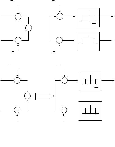
Let us now go back to the multipath fading channel (2.14) with impulse response given by (2.18). Let xbt and ybt be the complex baseband equivalents of the transmitted signal x t and the received signal y t, respectively. Figure 2.9 shows the system diagram from xbt to ybt. This implementation of a passband communication system is known as quadrature amplitude modulation (QAM). The signal xbt is sometimes called the
24
Figure 2.8 Illustration of upconversion from sb(t) to s(t), followed by downconversion from s(t) back to sb(t).
Figure 2.9 System diagram from the baseband transmitted signal xb(t) to the baseband received signal yb(t).
The wireless channel
√2 cos 2π fc t
[sb(t)] 
 X
X
+
[sb(t)]
 X
X
–√2 sin 2π fc t
√2 cos 2π fc t
[xb(t)]
X
+
[xb(t)]
 X
X
√2 cos 2π fc t
1 [sb(t)]
X
–W |
W |
2 |
2 |
 s(t)
s(t) 
1 [sb(t)]
 X
X
–W |
W |
2 |
2 |
–√2 sin 2π fc t
√2 cos 2π fc t
X |
1 |
[yb(t)] |
|
||
–W |
|
W |
2 |
|
2 |
x(t) y(t)  h(τ, t)
1 [yb(t)]  X
X 

–W |
W |
2 |
2 |
–√ |
|
sin 2π fc t |
–√ |
|
sin 2π fc t |
2 |
2 |
in-phase component I and xbt the quadrature component Q (rotated by /2). We now calculate the baseband equivalent channel. Substituting x t = √2 xbte j2 fct and y t = √2 ybte j2 fct into (2.14) we get
ybte j2 fct = i |
ait xbt − ite j2 fc t− i t |
|
(2.24) |
|||
= i |
ait xbt − ite−j2 fc i t e j2 fct |
|
||||
|
|
|
|
|
|
|
Similarly, one can obtain (Exercise 2.13) |
|
|
||||
ybte j2 fct = |
i |
ait xbt − ite−j2 fc i t e j2 fct |
|
(2.25) |
||
|
|
|
|
|
|
|
Hence, the baseband equivalent channel is |
|
|
||||
|
ybt = i |
aibt xbt − it |
|
(2.26) |
||

25 |
2.2 Input/output model of the wireless channel |
where
aib t = ai t e−j2 fc i t |
(2.27) |
The input/output relationship in (2.26) is also that of a linear time-varying system, and the baseband equivalent impulse response is
hb t = abi t − i t (2.28)
i
This representation is easy to interpret in the time domain, where the effect of the carrier frequency can be seen explicitly. The baseband output is the sum, over each path, of the delayed replicas of the baseband input. The magnitude of the ith such term is the magnitude of the response on the given path; this changes slowly, with significant changes occurring on the order of seconds or more. The phase is changed by /2 (i.e., is changed significantly) when the delay on the path changes by 1/ 4fc , or equivalently, when the path length changes by a quarter wavelength, i.e., by c/ 4fc . If the path length is changing at velocity v, the time required for such a phase change is c/ 4fcv . Recalling that the Doppler shift D at frequency f is fv/c, and noting that f ≈ fc for narrowband communication, the time required for a/2 phase change is 1/ 4D . For the single reflecting wall example, this is about 5 ms (assuming fc = 900 MHz and v = 60 km/h). The phases of both paths are rotating at this rate but in opposite directions.
Note that the Fourier transform Hb f t of hb t for a fixed t is simply H f + fc t , i.e., the frequency response of the original system (at a fixed t) shifted by the carrier frequency. This provides another way of thinking about the baseband equivalent channel.
2.2.3 A discrete-time baseband model
The next step in creating a useful channel model is to convert the continuoustime channel to a discrete-time channel. We take the usual approach of the sampling theorem. Assume that the input waveform is band-limited to W . The baseband equivalent is then limited to W/2 and can be represented as
xb t = |
|
|
x n sinc Wt − n |
(2.29) |
n
where x n is given by xb n/W and sinc t is defined as
sinc t = |
sin t |
|
(2.30) |
t |
This representation follows from the sampling theorem, which says that any waveform band-limited to W/2 can be expanded in terms of the orthogonal
26 The wireless channel
basis sincWt −nn, with coefficients given by the samples (taken uniformly at integer multiples of 1/W ).
Using (2.26), the baseband output is given by |
|
||
ybt = x n aibtsincWt − Wit − n |
(2.31) |
||
|
n |
i |
|
The sampled outputs |
at |
multiples of 1/W , y m = ybm/W , |
are then |
given by |
|
|
|
y m = x n aibm/W sincm − n − im/W W |
(2.32) |
||
n |
i |
|
|
The sampled output y m can equivalently be thought of as the projection of the waveform ybt onto the waveform W sincWt − m. Let = m − n. Then
y m = x m − aibm/W sinc − im/W W |
(2.33) |
||||
|
i |
|
|
|
|
By defining |
|
|
|
|
|
|
|
|
|
|
|
|
h m = i |
aibm/W sinc − im/W W |
|
(2.34) |
|
(2.33) can be written in the simple form |
|
||||
|
y m = |
h m x m − |
(2.35) |
||
We denote h m as the th (complex) channel filter tap at time m. Its value is a function of mainly the gains abi t of the paths, whose delays it are close to /W (Figure 2.10). In the special case where the gains abi t and the delays it of the paths are time-invariant, (2.34) simplifies to
h = abi sinc − iW (2.36)
i
and the channel is linear time-invariant. The th tap can be interpreted as the sample /W th of the low-pass filtered baseband channel response hb (cf. (2.19)) convolved with sinc(W).
We can interpret the sampling operation as modulation and demodulation in a communication system. At time n, we are modulating the complex symbol x m (in-phase plus quadrature components) by the sinc pulse before the up-conversion. At the receiver, the received signal is sampled at times m/W

27 |
2.2 Input/output model of the wireless channel |
Figure 2.10 Due to the decay of the sinc function, the ith path contributes most significantly to the th tap if its delay falls in the window
/W − 1/2W /W + 1/2W .
|
1 |
|
|
W |
|
i = 0 |
|
|
i = 1 |
|
|
i = 2 |
|
|
i = 3 |
|
|
i = 4 |
|
|
0 |
1 |
l |
2 |
Main contribution l = 0
Main contribution l = 0
Main contribution l = 1
Main contribution l = 2
Main contribution l = 2
at the output of the low-pass filter. Figure 2.11 shows the complete system. In practice, other transmit pulses, such as the raised cosine pulse, are often used in place of the sinc pulse, which has rather poor time-decay property and tends to be more susceptible to timing errors. This necessitates sampling at the Nyquist sampling rate, but does not alter the essential nature of the model. Hence we will confine to Nyquist sampling.
Due to the Doppler spread, the bandwidth of the output yb t is generally slightly larger than the bandwidth W/2 of the input xb t , and thus the output samples y m do not fully represent the output waveform. This problem is usually ignored in practice, since the Doppler spread is small (of the order of tens to hundreds of Hz) compared to the bandwidth W . Also, it is very convenient for the sampling rate of the input and output to be the same. Alternatively, it would be possible to sample the output at twice the rate of the input. This would recapture all the information in the received waveform.