52 2. Finite Field Arithmetic

The contribution by Sun Microsystems Laboratories (SML) to the OpenSSL project in 2002 provides a case study of the compromises chosen in practice. OpenSSL is widely used to provide cryptographic services for the Apache web server and the OpenSSH secure shell communication tool. SML’s contribution must be understood in context: OpenSSL is a public and collaborative effort—it is likely that Sun’s proprietary code has significant enhancements.

To keep the code size relatively small, SML implemented a fairly generic polynomial multiplication method. Karatsuba-Ofman is used, but only on multiplication of 2-word quantities rather than recursive application. At the lowest level of multiplication of 1-word quantities, a simplified Algorithm 2.36 is applied (with w = 2, w = 3, and w = 4 on 16-bit, 32-bit, and 64-bit platforms, respectively). As expected, the result tends to be much slower than the fastest versions of Algorithm 2.36. In our tests on Sun SPARC and Intel P6-family hardware, the Karatsuba-Ofman method implemented is less efficient than use of Algorithm 2.36 at the 2-word stage. However, the contribution from SML may be a better compromise in OpenSSL if the same code is used across platforms and compilers.

2.3.4Polynomial squaring

Since squaring a binary polynomial is a linear operation, it is much faster than multiplying two arbitrary polynomials; i.e., if a(z) = am−1zm−1 + · · · + a2 z2 + a1 z + a0, then

a(z)2 = am−1z2m−2 + · · · + a2 z4 + a1z2 + a0.

The binary representation of a(z)2 is obtained by inserting a 0 bit between consecutive bits of the binary representation of a(z) as shown in Figure 2.8. To facilitate this process, a table T of size 512 bytes can be precomputed for converting 8-bit polynomials into their expanded 16-bit counterparts. Algorithm 2.39 describes this procedure for the parameter W = 32.

Figure 2.8. Squaring a binary polynomial a(z) = am−1zm−1 + · · · + a2z2 + a1z + a0.

Algorithm 2.39 Polynomial squaring (with wordlength W = 32)

INPUT: A binary polynomial a(z) of degree at most m − 1.

OUTPUT: c(z) = a(z)2.

1.Precomputation. For each byte d = (d7, . . . , d1, d0), compute the 16-bit quantity

T (d) = (0, d7, . . . , 0, d1, 0, d0).

2.For i from 0 to t − 1 do

2.1Let A[i] = (u3, u2, u1, u0) where each u j is a byte.

2.2C[2i] ← (T (u1), T (u0)), C[2i + 1] ← (T (u3), T (u2)).

3.Return(c).

2.3.5Reduction

We now discuss techniques for reducing a binary polynomial c(z) obtained by multiplying two binary polynomials of degree ≤ m − 1, or by squaring a binary polynomial of degree ≤ m − 1. Such polynomials c(z) have degree at most 2m − 2.

Arbitrary reduction polynomials

Recall that f (z) = zm + r (z), where r (z) is a binary polynomial of degree at most m − 1. Algorithm 2.40 reduces c(z) modulo f (z) one bit at a time, starting with the leftmost bit. It is based on the observation that

c(z) = c2m−2z2m−2 + · · · + cm zm + cm−1zm−1 + · · · + c1z + c0

≡ (c2m−2zm−2 + · · · + cm )r (z) + cm−1zm−1 + · · · + c1z + c0 (mod f (z)).

The reduction is accelerated by precomputing the polynomials zkr (z), 0 ≤ k ≤ W − 1. If r (z) is a low-degree polynomial, or if f (z) is a trinomial, then the space requirements are smaller, and furthermore the additions involving zkr (z) in step 2.1 are faster. The following notation is used: if C = (C[n], . . . , C[2], C[1], C[0]) is an array, then C{ j } denotes the truncated array (C[n], . . . , C[ j + 1], C[ j ]).

Algorithm 2.40 Modular reduction (one bit at a time)

INPUT: A binary polynomial c(z) of degree at most 2m − 2.

OUTPUT: c(z) mod f (z).

1.Precomputation. Compute uk (z) = zkr (z), 0 ≤ k ≤ W − 1.

2.For i from 2m − 2 downto m do

2.1 If ci = 1 then

Let j = (i − m)/ W and k = (i − m) − W j . Add uk (z) to C{ j }.

3. Return(C[t − 1], . . . , C[1], C[0]).

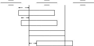
By considering the four columns on the right side of the above congruences, we see that reduction of C[9] can be performed by adding C[9] four times to C, with the rightmost bit of C[9] added to bits 132, 131, 128 and 125 of C; this is illustrated in Figure 2.9.

4

C[9]

3

C[9]

C[9]

Figure 2.9. Reducing the 32-bit word C[9] modulo f (z) = z163 + z7 + z6 + z3 + 1.

NIST reduction polynomials

We next present algorithms for fast reduction modulo the following reduction polynomials recommended by NIST in the FIPS 186-2 standard:

f (z) = z163 + z7 + z6 + z3 + 1

f (z) = z233 + z74 + 1

f (z) = z283 + z12 + z7 + z5 + 1

f (z) = z409 + z87 + 1

f (z) = z571 + z10 + z5 + z2 + 1.

These algorithms, which assume a wordlength W = 32, are based on ideas similar to those leading to Figure 2.9. They are faster than Algorithm 2.40 and furthermore have no storage overhead.

Algorithm 2.41 Fast reduction modulo f (z) = z163 + z7 + z6 + z3 + 1 (with W = 32)

INPUT: A binary polynomial c(z) of degree at most 324. OUTPUT: c(z) mod f (z).

1. For i from 10 downto 6 do

1.1T ← C[i].

1.2C[i − 6] ← C[i − 6] (T 29).

1.3C[i − 5] ← C[i − 5] (T 4) (T 3) T (T 3).

1.4C[i − 4] ← C[i − 4] (T 28) (T 29).

3.C[0] ← C[0] (T 7) (T 6) (T 3) T .

4.C[1] ← C[1] (T 25) (T 26).

Algorithm 2.42 Fast reduction modulo f (z) = z233 + z74 + 1 (with W = 32)

INPUT: A binary polynomial c(z) of degree at most 464. OUTPUT: c(z) mod f (z).

1. For i from 15 downto 8 do

1.1T ← C[i].

1.2C[i − 8] ← C[i − 8] (T 23).

1.3C[i − 7] ← C[i − 7] (T 9).

1.4C[i − 5] ← C[i − 5] (T 1).

1.5C[i − 4] ← C[i − 4] (T 31).

2. T ← C[7] 9.

3.C[0] ← C[0] T .

4.C[2] ← C[2] (T 10).

5.C[3] ← C[3] (T 22).

56 2. Finite Field Arithmetic

Algorithm 2.43 Fast reduction modulo f (z) = z283 + z12 + z7 + z5 + 1 (with W = 32)

INPUT: A binary polynomial c(z) of degree at most 564. OUTPUT: c(z) mod f (z).

1. For i from 17 downto 9 do

1.1T ← C[i].

1.2C[i − 9] ← C[i − 9] (T 5) (T 10) (T 12) (T 17).

1.3C[i − 8] ← C[i − 8] (T 27) (T 22) (T 20) (T 15).

Algorithm 2.44 Fast reduction modulo f (z) = z409 + z87 + 1 (with W = 32)

INPUT: A binary polynomial c(z) of degree at most 816. OUTPUT: c(z) mod f (z).

1. For i from 25 downto 13 do

1.1T ← C[i].

1.2C[i − 13] ← C[i − 13] (T 7).

1.3C[i − 12] ← C[i − 12] (T 25).

1.4C[i − 11] ← C[i − 11] (T 30).

1.5C[i − 10] ← C[i − 10] (T 2).

3.C[0] ← C[0] T .

4.C[2] ← C[2] (T¡¡23).

Algorithm 2.45 Fast reduction modulo f (z) = z571 + z10 + z5 + z2 + 1 (with W = 32)

INPUT: A binary polynomial c(z) of degree at most 1140. OUTPUT: c(z) mod f (z).

1. For i from 35 downto 18 do

1.1T ← C[i].

1.2C[i − 18] ← C[i − 18] (T 5) (T 7) (T 10) (T 15).

1.3C[i − 17] ← C[i − 17] (T 27) (T 25) (T 22) (T 17).

2.3.6Inversion and division

In this subsection, we simplify the notation and denote binary polynomials a(z) by a. Recall that the inverse of a nonzero element a F2m is the unique element g F2m such that ag = 1 in F2m , that is, ag ≡ 1 (mod f ). This inverse element is denoted a−1 mod f or simply a−1 if the reduction polynomial f is understood from context. Inverses can be efficiently computed by the extended Euclidean algorithm for polynomials.

The extended Euclidean algorithm for polynomials

Let a and b be binary polynomials, not both 0. The greatest common divisor (gcd) of a and b, denoted gcd(a, b), is the binary polynomial d of highest degree that divides both a and b. Efficient algorithms for computing gcd(a, b) exploit the following polynomial analogue of Theorem 2.18.

Theorem 2.46 Let a and b be binary polynomials. Then gcd(a, b) = gcd(b − ca, a) for all binary polynomials c.

In the classical Euclidean algorithm for computing the gcd of binary polynomials a and b, where deg(b) ≥ deg(a), b is divided by a to obtain a quotient q and a remainder r satisfying b = qa + r and deg(r ) < deg(a). By Theorem 2.46, gcd(a, b) = gcd(r, a). Thus, the problem of determining gcd(a, b) is reduced to that of computing gcd(r, a) where the arguments (r, a) have lower degrees than the degrees of the original arguments (a, b). This process is repeated until one of the arguments is zero—the result is then immediately obtained since gcd(0, d) = d. The algorithm must terminate since the degrees of the remainders are strictly decreasing. Moreover, it is efficient because the number of (long) divisions is at most k where k = deg(a).

In a variant of the classical Euclidean algorithm, only one step of each long division is performed. That is, if deg(b) ≥ deg(a) and j = deg(b) − deg(a), then one computes

r = b + z j a. By Theorem 2.46, gcd(a, b) = gcd(r, a). This process is repeated until a zero remainder is encountered. Since deg(r ) < deg(b), the number of (partial) division steps is at most 2k where k = max{deg(a), deg(b)}.

The Euclidean algorithm can be extended to find binary polynomials g and h satisfying ag + bh = d where d = gcd(a, b). Algorithm 2.47 maintains the invariants

ag1 + bh1 = u ag2 + bh2 = v.

The algorithm terminates when u = 0, in which case v = gcd(a, b) and ag2 + bh2 = d.

58 2. Finite Field Arithmetic

Algorithm 2.47 Extended Euclidean algorithm for binary polynomials

INPUT: Nonzero binary polynomials a and b with deg(a) ≤ deg(b).

OUTPUT: d = gcd(a, b) and binary polynomials g, h satisfying ag + bh = d.

1.u ← a, v ← b.

2.g1 ← 1, g2 ← 0, h1 ← 0, h2 ← 1.

3.While u = 0 do

3.1j ← deg(u) − deg(v).

3.2If j < 0 then: u ↔ v, g1 ↔ g2, h1 ↔ h2, j ← − j .

3.3u ← u + z j v.

3.4g1 ← g1 + z j g2, h1 ← h1 + z j h2.

4.d ← v, g ← g2, h ← h2.

5.Return(d, g, h).

Suppose now that f is an irreducible binary polynomial of degree m and the nonzero polynomial a has degree at most m − 1 (hence gcd(a, f ) = 1). If Algorithm 2.47 is executed with inputs a and f , the last nonzero u encountered in step 3.3 is u = 1. After this occurrence, the polynomials g1 and h1, as updated in step 3.4, satisfy ag1 + f h1 = 1. Hence ag1 ≡ 1 (mod f ) and so a−1 = g1. Note that h1 and h2 are not needed for the determination of g1. These observations lead to Algorithm 2.48 for inversion in F2m .

Algorithm 2.48 Inversion in F2m using the extended Euclidean algorithm

INPUT: A nonzero binary polynomial a of degree at most m − 1.

OUTPUT: a−1 mod f .

1.u ← a, v ← f .

2.g1 ← 1, g2 ← 0.

3.While u = 1 do

3.1j ← deg(u) − deg(v).

3.2If j < 0 then: u ↔ v, g1 ↔ g2, j ← − j .

3.3u ← u + z j v.

3.4g1 ← g1 + z j g2.

4.Return(g1).

Binary inversion algorithm

Algorithm 2.49 is the polynomial analogue of the binary algorithm for inversion in F p (Algorithm 2.22). In contrast to Algorithm 2.48 where the bits of u and v are cleared from left to right (high degree terms to low degree terms), the bits of u and v in Algorithm 2.49 are cleared from right to left.

Algorithm 2.49 Binary algorithm for inversion in F2m

INPUT: A nonzero binary polynomial a of degree at most m − 1.

OUTPUT: a−1 mod f .

1.u ← a, v ← f .

2.g1 ← 1, g2 ← 0.

3.While (u = 1 and v = 1) do

3.1While z divides u do u ← u/z.

If z divides g1 then g1 ← g1/z; else g1 ← (g1 + f )/z.

3.2While z divides v do v ← v/z.

If z divides g2 then g2 ← g2/z; else g2 ← (g2 + f )/z.

3.3If deg(u) > deg(v) then: u ← u + v, g1 ← g1 + g2; Else: v ← v + u, g2 ← g2 + g1.

4.If u = 1 then return(g1); else return(g2).

The expression involving degree calculations in step 3.3 may be replaced by a simpler comparison on the binary representations of the polynomials. This differs from Algorithm 2.48, where explicit degree calculations are required in step 3.1.

Almost inverse algorithm

The almost inverse algorithm (Algorithm 2.50) is a modification of the binary inversion algorithm (Algorithm 2.49) in which a polynomial g and a positive integer k are first computed satisfying

ag ≡ zk (mod f ).

A reduction is then applied to obtain

a−1 = z−k g mod f.

The invariants maintained are

ag1 + f h1 = zk u ag2 + f h2 = zk v

for some h1, h2 that are not explicitly calculated.

60 2. Finite Field Arithmetic

Algorithm 2.50 Almost Inverse Algorithm for inversion in F2m

INPUT: A nonzero binary polynomial a of degree at most m − 1.

OUTPUT: a−1 mod f .

1.u ← a, v ← f .

2.g1 ← 1, g2 ← 0, k ← 0.

3.While (u = 1 and v = 1) do

3.1While z divides u do

u ← u/z, g2 ← z · g2, k ← k + 1. 3.2 While z divides v do

v ← v/z, g1 ← z · g1, k ← k + 1.

3.3 If deg(u) > deg(v) then: u ← u + v, g1 ← g1 + g2. Else: v ← v + u, g2 ← g2 + g1.

reduction polynomial f is said to be suitable if l is above some threshold (which may depend on the implementation; e.g., l ≥ W is desirable with W -bit words), since then less effort is required in the reduction step.

Steps 3.1–3.2 are simpler than those in Algorithm 2.49. In addition, the g1 and g2 appearing in these algorithms grow more slowly in almost inverse. Thus one can expect Algorithm 2.50 to outperform Algorithm 2.49 if the reduction polynomial is suitable, and conversely. As with the binary algorithm, the conditional involving degree calculations may be replaced with a simpler comparison.

Division

The binary inversion algorithm (Algorithm 2.49) can be easily modified to perform division b/a = ba−1. In cases where the ratio I/M of inversion to multiplication costs is small, this could be especially significant in elliptic curve schemes, since an elliptic curve point operation in affine coordinates (see §3.1.2) could use division rather than an inversion and multiplication.

Division based on the binary algorithm To obtain b/a, Algorithm 2.49 is modified at step 2, replacing g1 ← 1 with g1 ← b. The associated invariants are

ag1 + f h1 = ub ag2 + f h2 = vb.

On termination with u = 1, it follows that g1 = ba−1. The division algorithm is expected to have the same running time as the binary algorithm, since g1 in Algorithm 2.49 goes to full-length in a few iterations at step 3.1 (i.e., the difference in initialization of g1 does not contribute significantly to the time for division versus inversion).

If the binary algorithm is the inversion method of choice, then affine point operations would benefit from use of division, since the cost of a point double or addition changes from I + 2M to I + M. (I and M denote the time to perform an inversion and a multiplication, respectively.) If I/M is small, then this represents a significant improvement. For example, if I/M is 3, then use of a division algorithm variant of Algorithm 2.49 provides a 20% reduction in the time to perform an affine point double or addition. However, if I/M > 7, then the savings is less than 12%. Unless I/M is very small, it is likely that schemes are used which reduce the number of inversions required (e.g., halving and projective coordinates), so that point multiplication involves relatively few field inversions, diluting any savings from use of a division algorithm.

Division based on the extended Euclidean algorithm Algorithm 2.48 can be transformed to a division algorithm in a similar fashion. However, the change in the initialization step may have significant impact on implementation of a division algorithm variant. There are two performance issues: tracking of the lengths of variables, and implementing the addition to g1 at step 3.4.

In Algorithm 2.48, it is relatively easy to track the lengths of u and v efficiently (the lengths shrink), and, moreover, it is also possible to track the lengths of g1 and g2. However, the change in initialization for division means that g1 goes to full-length immediately, and optimizations based on shorter lengths disappear.

The second performance issue concerns the addition to g1 at step 3.4. An implementation may assume that ordinary polynomial addition with no reduction may be performed; that is, the degrees of g1 and g2 never exceed m −1. In adapting for division, step 3.4 may be less-efficiently implemented, since g1 is full-length on initialization.

Division based on the almost inverse algorithm Although Algorithm 2.50 is similar to the binary algorithm, the ability to efficiently track the lengths of g1 and g2 (in addition to the lengths of u and v) may be an implementation advantage of Algorithm 2.50 over Algorithm 2.49 (provided that the reduction polynomial f is suitable). As with Algorithm 2.48, this advantage is lost in a division algorithm variant.

It should be noted that efficient tracking of the lengths of g1 and g2 (in addition to the lengths of u and v) in Algorithm 2.50 may involve significant code expansion (perhaps t2 fragments rather than the t fragments in the binary algorithm). If the expansion cannot be tolerated (because of application constraints or platform characteristics), then almost inverse may not be preferable to the other inversion algorithms (even if the reduction polynomial is suitable).

62 2. Finite Field Arithmetic

2.4Optimal extension field arithmetic

Preceding sections discussed arithmetic for fields F pm in the case that p = 2 (binary fields) and m = 1 (prime fields). As noted on page 28, the polynomial basis representation in the binary field case can be generalized to all extension fields F pm , with coefficient arithmetic performed in F p.

For hardware implementations, binary fields are attractive since the operations involve only shifts and bitwise addition modulo 2. The simplicity is also attractive for software implementations on general-purpose processors; however the field multiplication is essentially a few bits at a time and can be much slower than prime field arithmetic if a hardware integer multiplier is available. On the other hand, the arithmetic in prime fields can be more difficult to implement efficiently, due in part to the propagation of carry bits.

The general idea in optimal extension fields is to select p, m, and the reduction polynomial to more closely match the underlying hardware characteristics. In particular, the value of p may be selected to fit in a single word, simplifying the handling of carry (since coefficients are single-word).

Definition 2.51 An optimal extension field (OEF) is a finite field F pm such that:

1.p = 2n − c for some integers n and c with log2 |c| ≤ n/2; and

2.an irreducible polynomial f (z) = zm − ω in F p [z] exists.

If c {±1}, then the OEF is said to be of Type I ( p is a Mersenne prime if c = 1); if ω = 2, the OEF is said to be of Type II.

Type I OEFs have especially simple arithmetic in the subfield F p , while Type II OEFs allow simplifications in the F pm extension field arithmetic. Examples of OEFs are given in Table 2.1.

Table 2.1. OEF example parameters. Here, p = 2n − c is prime, and f (z) = zm − ω F p[z] is irreducible over F p. The field is F pm = F p[z]/( f ) of order approximately 2mn .

The following results can be used to determine if a given polynomial f (z) = zm − ω is irreducible in F p[z].