Table 4.1 Procedure for Determining Load Allocation for Two Units Whose Curves Are Shown in Fig. 4-2*

(1)	(2)	(3)	(4)	(5)
			Charge	Incremental
			for load	rate,
Load,	Million	Dollars/h	increment,	dollars/MWh
MW	- Btu/h	(2) X $3.50	dollars/h	(4) - (1)

Unit A

incremental Rates 3

Economic Loading of Generating Units 25

s _ 35

s в 35

Computers for Economic Loading 37

Effects of Varying Fuel Costs 38

Nuclear Generation 38

Geothermal Generation 38

Solar and Wind Generation 39

Coordination of Hydro and Thermal Generation 39

Transmission Losses 41

Economic Interchange of Power 43

Summary 53

Problems 55

Power System Control 58

Introduction 58

Power System Control Elements 59

Automatic Generation Control 60

Interconnected Operation 61

Modes of Tie-Line Operation 62

Tie-Line Bias 63

Area Control Error 42

Accumulated Frequency Error 42

Summary 43

Problems 43

0	250	875
20	350	1225	350	17.50
40	450	1575	350	17.50
60	600	2100	525	26.20
80	800	2800	700	35.00
100	1050	3675*	875	43.80

*The fuel costs shown in this tabulation have been increased by a factor of 10 to more realisti­cally reflect present costs, which have drastically increased since the first edition was prepared.

units whose input-output curves are shown in Fig. 4-2 is shown in Table 4-1. Since we are primarily interested in cost, the fuel rates will be converted to dollars per hour for various loads. The incremental rate in dollars per megawatthour for various loads is determined. A fuel price of $3.50 per million Btu is assumed.*

Figure 4-5Input-output curves showing fuel dollars per hour versus MW load.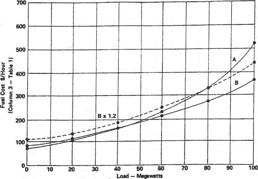

О 10 20 30 40 50 60 70 80 90 100 Load — Megawatts

Figure 4-6Incremental cost curves for units A and B.

10.00

X

s _

? ~Z 8.00

м

| » 6.00 с

s в

II

I 3 4.00

оj:

0

2.00'

The incremental-rate information developed in Table 4-1 can be plotted as curves for both machines (Figs. 4-5 and 4-6). If 1-h peri­ods are considered, the vertical scale will be incremental cost in dol­lars per megawatthour, with megawatts as the horizontal scale, as shown in Fig. 4-6.

	Unit A			Unit В
	Incr.			Incr.
	fuel			fuel		Total
	cost,	Fuel		cost,	Fuel	fuel
Load,	dollars/	cost,	Load,	dollars/	cost,	cost,
MW	MWh	dollars/h	MW	MWh	dollars/h	dollars/h
0	15.50	730.00	100	48.50	3650.00	4380.00
10	17.50	830.00	90	43.80	3220.00	4050.00
20	21.00	1010.00	80	39.00	2800.00	3810.00
30	26.30	1250.00	70	35.00	2450.00	3700.00
40	30.00	1575.00	60	30.00	2100.00	3670.00
50	35.00	1870.00	50	26.50	1825.00	3695.00
60	43.00	2250.00	40	21.00	1575.00	3820.00
70	52.50	2750.00	30	17.50	1400.00	4150.00
80	66.00	3320.00	20	17.50	1228.00	4540.00
90	96.50	4100.00	10	17.50	1050.00	5150.00
100	—	5200.00	0	17.50	900.00	6100.00

From the information shown in Figs. 4-5 and 4-6 it should be possible to determine the -proper division of load between the two machines to result in minimum fuel cost. Assume a total load of 100 MW to be car­ried by the two units. Various combinations of loading can be made, but the objective is to carry the load with minimum cost. The tabulation shown in Table 4-2 was developed by taking points on the incremental fuel-cost curves of Fig. 4-6 to match various load conditions and fuel cost per hour from the input-output curves shown in Fig. 4-5, where fuel cost in dollars per hour is plotted against loads in megawatts.

From Table 4-2 it can be seen that the minimum fuel cost occurs when unit A is loaded to 40 MW and unit Вto 60 MW with incremen­tal costs of $30 MWh for each machine. If desired, tabulations similar to that in Table 4-2 can be set up for other fuel costs and the mini­mum cost (fuel rates) determined as further proof of the principle of loading machines for equal incremental costs.

It is obvious that when many units are involved, a manual solution of the economic loading problem is impractical, because many load changes would be needed while solving the problem for only one situ­ation. Various devices have been developed to help solve the economic loading problem rapidly where many generating units are involved.

Probably the simplest device for allocating load on an incremental basis was the incremental loading slide rule. These devices were used to a considerable extent prior to the advent of digital computers and the development of computerized economic loading programs. These slide rules made use of sliding elements showing unit loading on loga­rithmic scales, and a straightedge that could be adjusted in position. The sliding elements could be set to the unit fuel cost, and by moving the straightedge to the appropriate position, unit loadings could be determined for minimum overall fuel cost.

Computers for Economic Loading

Digital computers are almost universally used for calculating econom­ic loading of generating units. Although there may still be some ana­log load-frequency-control (LFC) systems in use, they are rapidly being supplanted by digital systems.

The particular advantage of computers is that they can continu­ously monitor the system loading conditions, determine the most economical allocation of generation between units, and send control impulses to load the units to the desired values. Computer control, properly applied, can approach an almost exact allocation of unit loadings for minimum fuel cost. In applying computers to online eco­nomic loading problems, the unit input-output curves and incre- mental-fuel-rate curves are stored in the computer, which goes through a process similar to that followed in Table 4-2 to calculate the desired machine loadings. Because of the tremendous speed at which computations can be made in a digital computer, it can solve economic loading problems in very short time intervals and simulta­neously carry out other system-control functions.

Automatic generation control (AGO) is commonly included in super­visory control and data acquisition system (SCADA) installations. Such systems are described in Chap. 8.

Effects of Varying Fuel Costs

Before leaving the problem of incremental loading of thermal plants, the matter of varying fuel costs should be mentioned. The shapes of the input-output and incremental-fuel-rate curves are not changed by different fuels or by changes in the cost of the same fuel. Consequently, if the incremental curves are plotted with incremental cost as the vertical scale, the ratio of the cost of the fuel being burned to the cost of the fuel for which the curves were drawn can be used as a multiplying factor. This factor is employed to correct for fuel-cost changes for any or all of the units. By this means it is possible to solve the economic loading problem under all conditions of fuel cost.

There is a further complication, which is accounting for losses due to transmission of power from generation to load. This will be dis­cussed in more detail later. It will suffice for the moment to state that transmission losses can be, and are, evaluated and their effect used as a multiplier (called a penalty factor) on the incremental cost of power from each plant or unit to convert the plant incremental cost to a load center incremental cost.

By determining the cost of power from each source, including the cost of transporting it to the load center, it is possible to compare the actual costs of power from the various sources and, within lim­its, to adjust loadings so that the incremental costs from all sources are equal. Optimization methods demonstrate that minimum cost of power to the system is achieved when the incremental costs from all sources are equal.

The penalty factors of remote plants can exceed 1.1 and those for load center plants can be less than 0.9. The determination of the penalty factor and its application to the loading of generation and purchase sources can be significant in the economic operation of a power system.

Nuclear Generation

The above discussion has been confined to the loading of conventional fossil-fueled thermal plants. Nuclear plants present a special situation since the incremental production costs are quite low compared to fossil- fueled plants. The total energy that can be produced by a nuclear reac­tor is maximized if it is operated at a relatively constant load; conse­quently, such units are generally designed to be base-loaded.

Geothermal Generation

As a result of escalating fuel costs in recent years, there has been greatly increased interest in the use of geothermal energy for electric power generation. This source can only be used where there are sources of natural steam or hot water that can be economically devel­oped. The largest such development is the Geysers geothermal devel­opment in Northern California with a total capacity of approximately 1000 MW. This plant is made up of many generating units in the 50- to 100-MW range with steam supplied from nearby steam wells asso­ciated with the units. This avoids the heat losses that would occur if it were attempted to pipe the steam over significant distances. In order to minimize air and water pollution, after passing through the turbines, the steam is condensed and the condensate is returned to the ground into wells drilled for that purpose.

Like nuclear installations, the units at geothermal plants are nor­mally operated as base-load units and not on an incremental basis.

Solar and Wind Generation

There has been considerable interest in the past few years in the development of electrical power without using fossil fuels, and using sources that are nonpolluting to the atmosphere. Efforts have been directed in the development of solar energy and wind power into eco­nomical sources, and with capacities great enough to be significant as commercial power producers.

Progress has been made in both areas, and there are installations of both types in service. However, there are still size limitations, and both solar and wind power installations are dependent upon the avail­ability of favorable sun and wind conditions, which are of course quite variable and cannot be considered to be base-load sources. Incremental loading techniques are not adaptable to either of these sources; howev­er, to the extent that power from solar and wind sources is available, they will reduce dependence upon normal fossil fuels.

Coordination of Hydro and Thermal Generation

The operation of hydro units in a system in which both hydro and ther­mal generation are used presents an extension of the economic loading problem. There are many conditions connected with hydro operation, such as uncontrolled flows and required releases of water for irrigation, flood control, salinity control, and other needs that may be imposed by governmental agencies and that take away from the system operator some of the alternatives that might be available if the water could be used entirely as desired for the benefit of power production. However, if a value can be placed on water in each reservoir, usually in dollars per acre-foot, hydro units can be operated incrementally along with ther­mal units for overall economic operation of the system.

Of course the value of water changes from time to time, being lower when the cost of alternative sources is lower and during periods of high flow, such as during and immediately following storms, and increased when alternative costs are high and during periods when flows are low or when reservoirs are being drafted at controlled rates of flow. Since each acre-foot of water through a hydro plant will develop a definite amount of electrical energy, depending on the head of the plant, water is equivalent to fuel such as gas or oil for power-producing purposes.

Procedures for integrating the operation of hydro and thermal gener­ation on a system for minimum cost of generation have been developed and are in use. This procedure is called hydrothermal coordination.

Basically in a hydrothermal-coordination program, input-output curves for each hydro unit are developed, showing acre-feet per hour plotted against load in megawatts. From the input-output curves the incremental water rate in acre-feet per megawatthour plotted against the load in megawatts can be developed by exactly the same method used for thermal plants.

An arbitrary price in dollars per acre-foot is placed on the water for each plant. If it is desired to use more water, the price is reduced, and

if less water is to be used, the water price is increased. By proper selection of water prices, exactly the desired amount of water will be used in any desired time period. The hydro plants then will follow incremental loading requirements and help achieve the desired result of overall minimum fuel cost.

The water value in hydrothermal coordination programs is usual­ly denoted by the Greek letter gamma (y) to distinguish it from the thermal unit and system fuel cost, which is designated by the Greek letter lambda (A).

The proper integration of hydro and thermal generation for mini­mum overall cost is quite complex and can be solved optimally only by a digital computer. Even with a computer, the number of calcula­tions used to determine the most economic operation can be so great that considerable computer time is required to obtain a correct solu­tion to the problem.

Transmission Losses

The preceding discussion has centered on determining the loads to be placed on thermal and hydro units in order to obtain equal incremental fuel cost for minimum overall cost of generation. The problem is only partially solved, however, until transmission losses are considered.

It was mentioned previously that if transmission losses could be evaluated, their effect could be used as a multiplier on fuel cost (or water value for hydro) to compensate for the energy lost in transmis­sion and to arrive at a true economic loading of the system.

In the sections on energy transfer and var flows, it was pointed out that all transmission lines have resistance, determined by the con­ductor material, conductor size, and length of the line. It was also pointed out that the transmission loss in watts was the product of the line current squared times the resistance of the line (PR).

Lood

Ю0А -10 Ohms

Figure 4-7Simple transmission system of a single generator and load connected by a line carrying 100 A through 10О. Loss is equal to (100)²X 10 = 100,000 W or 100 kW.

In the simplest possible system, a generating unit connected by a single transmission line to a load, the determination of transmission loss is quite simple. Figure 4-7 illustrates this case.

The generator must, of course, produce enough energy to supply the load plus the transmission losses—in the above case, the load plus 100 kW. The power required to supply the losses will move the gener­ation to a higher point on the incremental cost curve, resulting in an increase in the cost of each kilowatthour of energy.

When two or more generating units are connected to a load via sep­arate transmission lines, the correct allocation of load between the units will result when the incremental costs, including the costs of supplying the energy for transmission losses, are equal.

Here again the problem rapidly compounds in complexity as the number of generators, lines, loads, and tie points is increased. Manual methods of calculating loss factors become impractical, and it is necessary to resort to analog or digital computing devices to deter­mine the effects of transmission losses on a power system.

No effort will be made here to develop the mathematical solution of the transmission loss problem. For the purposes of this discussion, it should suffice to state that a coordination equation has been devel­oped to determine what is called the penalty factor.Penalty factor is equal to 1/(1 — loss factor), and it can be seen that as the loss factor increases, the penalty factor will increase.

In order to determine penalty factors, it is necessary to develop a mathematical model of the system. After this has been done, an ana­log penalty-factor computer or a digital computer can be used to determine penalty factors for any load condition for each generating station or tie-line source to the system load center. When penalty-fac­tor calculations are made "off line," they are manually applied to incremental slide-rule slides for each unit or to penalty-factor setters on analog dispatch-control units. By this means the incremental-cost curves are adjusted upward or downward as required by the penalty factor so that the generating units are loaded on a strictly competitive basis for minimum cost, including transmission losses. These meth­ods have become relatively obsolete because of the wide acceptance and application of digital computers for power system control.

When digital computers are used for system control, penalty-factor calculations are made at frequent time intervals, and generation-con­trol impulses are produced, including current penalty factors, so that the system generation is consistently maintained with the most eco­nomic allocation between generating units.

It has been shown previously that minimum fuel input occurs when generating units are operated at equal incremental costs. To demon­strate the effect of transmission penalty factors on load division between generating units, an example will be worked out using the two machines previously considered, but with a penalty factor of 1.2 applied to unit Вand a penalty factor of 1.0 applied to unit A.

Under these conditions the values shown on the input-output and incremental-cost curves of unit Вwill be multiplied by 1.2 and replot- ted. This has been done, and the curves for unitВoperating with the assumed penalty factor are shown as the dashed curves on Figs. 4-5 and 4-6. The effect is to raise both the input-output and incremental- cost curves. If the penalty factor had been less than 1, it would indi­cate that system losses would be reduced by adding load to unit B, and the curves would move downward.

The comparative tabulation under the new operating conditions is shown in Table 4-3. This table shows that the minimum fuel cost occurs with 47 MW on unit Aand 53 MW on unit B,with an equal incremental fuel cost of $33/MWh.

Economic Interchange of Power

Another problem that is encountered by a system operator is to deter­mine when it is economical to buy power from or sell power to other systems. Whenever power is purchased and received into a system, the power that must be produced to carry the system load is reduced by the amount of power received from the other system. Conversely, whenever power is sold, power production must equal the system load plus the amount of the sale.

The preceding discussion has demonstrated that when the power output of generating units is increased, the unit incremental cost and also the system incremental cost (A) increase. Conversely, when