

In each cluster, find the sample variance:,
where  .
.
Then, to
test the hypothesis ![]() the criterion of the equality G Bartlett dispersions.
the criterion of the equality G Bartlett dispersions.
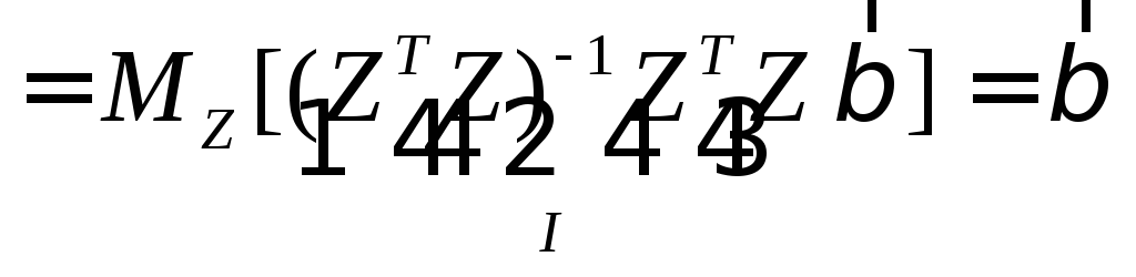
If ![]() is rejected, we use OLS:
is rejected, we use OLS:
![]() ,
where g –
cluster number to which it belongs n.
,
where g –
cluster number to which it belongs n.
2) autocorrelated errors.
It may be, for example, errors associated autoregression model of the 1st order (ar (1)):
![]() ,
,
![]() –white noise:
–white noise:
![]() ,
,
![]() ,
,
![]() –Kronecker
delta.
–Kronecker
delta.
 (autocorrelation
decay with increasing lag),
(autocorrelation
decay with increasing lag),
![]() .
.
Note: to test the hypothesis about the presence / absence of autocorrelation of errors (criterion Durbin - Watson)

![]() .
.
the test
statistic:  ,
,

Obvious
that ![]()
 , so,
if:
, so,
if:
1)
![]() ;
;
2)
![]() .
.
So that,
![]() ?
?
![]()
![]() ?
?
![]()
 | |
| | |
| |
| | |
![]()
![]() 2
2
![]()
![]() .
.
If there is
autocorrelation, а ![]() is unknown, it is possible:
is unknown, it is possible:
а) roughly
assume that ![]() (and substitute it in
(and substitute it in ![]() );
);
б) Use the procedure Cochrane - Orcutt:
–find
![]() ;
;
–
![]() ;
;
– value
![]() as is the OLS estimator of the regression coefficient in the model
as is the OLS estimator of the regression coefficient in the model
![]() ;
;
–
![]() ;
;
To continue
the cycle until ![]() stabilizes.
stabilizes.
The
disadvantage of the algorithm is that there is a risk to go to a
local minimum ![]() .
.
Prognosis OLMMR
Evaluation of a new yN (T) according to known factors produced by the formulas:
1. Heteroscedastic errors:
![]() .
.
2. Autocorrelated errors:
![]() .
.
Dichotomous resultant parameters. Logit and probit models
Often the dependent variable - the variable is binary otklika- in nature, ie. E. Can take only two values. For example, the patient may recover, but maybe not, the candidate for the post can go, and can fail the test when applying for a job, the person may be unemployed, and maybe have a job and so on. N. In all these cases, we may want to search according to between one or more "continuous" variables (for example, in the latter case x1 - age, x2 - income in the last year, x3 - work experience and so on. n.) and one dependent upon them a binary variable.
Of course, you can use standard multiple regression and compute the standard regression coefficients. For example, a variable can be set to the values y 1 'and 0, where 1 indicates that the corresponding person is unemployed, and 0 - it is busy. But here comes the problem: multiple regression "does not know" that the response variable is binary in nature. Therefore, it will inevitably lead to a model with predicted values greater than 1 and less than 0. But these values do not permissible for the original problem, so multiple regression ignores restrictions on the range of values for y.
Regression
problem can be formulated differently: instead of describing a binary
variable, we describe a continuous variable with values in the
interval [0, 1], which is interpreted as the probability
![]() .
(4)
.
(4)
Here ![]() – vector of covariates,
– vector of covariates, ![]() – vector of regression coefficients.
– vector of regression coefficients.
 –logistic
function.
–logistic
function.
Easy to see
that regardless of the regression coefficients and values ![]() p values will always belong to the segment [0, 1]:
p values will always belong to the segment [0, 1]:

Thus, the model logit regression has the form
![]() ,
(5)
,
(5)
where En - random error in the n-th dimension. obviously,
En
heteroscedasticity, since their dispersion depends on the ![]() .
.
If, instead
of ![]() use
use ![]() – the function of the standard normal distribution, it is probit
model.
– the function of the standard normal distribution, it is probit
model.
Model (5)
is nonlinear in the parameters And
before applying OLS should be linearized. Will move to the left and
the error is applicable to both sides of the inverse transformation
to ![]() .
Only the first terms of the expansion of the left by Taylor's
formula, we obtain:
.
Only the first terms of the expansion of the left by Taylor's
formula, we obtain:
![]() ,
,
where ![]() ,
error heteroscedasticity.
,
error heteroscedasticity.
To the
practical application of the MNE last expression to be meaningful,
must be considered grouped or duplicate data, replacing ![]() the average value is not equal to 0 and 1.
the average value is not equal to 0 and 1.
Due to the above difficulties, an assessment of the vector of regression coefficients is better to find the maximum likelihood method. If the probability of getting 1 is (4), the probability of getting 0 is 1- p and the probability of obtaining a chain of 1, 0, 0, ... is the product of the probability p (1-p) (1-p) ....
The likelihood function is:

The result
is determined by ![]() such that the probability of getting at the available factors
available responses will be maximum. To check the quality of the
simulation (the significance of the effects of factors) to test the
hypothesis
such that the probability of getting at the available factors
available responses will be maximum. To check the quality of the
simulation (the significance of the effects of factors) to test the
hypothesis
The test statistic - logarithm of the square of the likelihood ratio for models H1 and H0 - is under H0 is approximately chi-square distribution with K degrees of freedom, so the level of significance:
 .
.
The marginal effect of the factor
The marginal effect of factor xi shows the change in the probability
{Y = 1} xi factor changing unit.
Can show that it has the form:
 .
.
Example (continued): the percentage will increase the probability of success in the task with increasing experience (from its mean value = 16.88 m.) At 1 month?
Marginal effect = 0.4 * 0.6 * 0.161 = 0.038, ie, the probability of success is increased by 0.038, or about 10%.
Stochastic Explanatory Variables
This model has the form
![]() ,
(6)
,
(6)
Where now
![]() –
random variables;
–
random variables;

Z - random matrix plan.
We consider three cases.
1. Random
errors ![]() doesn’t depend from
doesn’t depend from ![]() .
.
In this case, all the results of the usual regression analysis retained. In particular, the OLS estimator is unbiased.
proof:![]()
![]()

 .
.
2 Random
errors depend on![]() .
.
![]() ,
and evaluation
,
and evaluation ![]() – biased and inconsistent.
– biased and inconsistent.
The method
of instrumental variables. Suppose that there are some variables
![]() ,
correlated with
,
correlated with![]() and independent with
and independent with ![]() ,
– "Instrumental variables":
,
– "Instrumental variables":
 ;
;
![]() ;
;
![]() ;
;
![]() ;
;
![]() –consistent
estimate of the coefficient vector in (6).
–consistent
estimate of the coefficient vector in (6).
Note: a similar way could be "print" and the usual formula of OLS.
Example (model Keynes):
![]() –consumption
in the country in the ith year;
–consumption
in the country in the ith year;
![]() –aggregate
output;
–aggregate
output;
![]() –random
feature th year;
–random
feature th year;
![]() –investment.
–investment.
 (7, 8)
(4) –> (5):
 .
.
It can be
seen that ![]() Dependds on
Dependds on ![]() ,
so
,
so ![]() ,
estimated according to equation (7), - biased and inconsistent. Lets
take
,
estimated according to equation (7), - biased and inconsistent. Lets
take ![]() as an instrument by: (8) it is correlated with not dependent, as
investment - an exogenous variable, and is determined by other
factors (maybe the political decisions) than
as an instrument by: (8) it is correlated with not dependent, as
investment - an exogenous variable, and is determined by other
factors (maybe the political decisions) than ![]() :
:
![]() .
.
Example: measurement of non-random variables (factors) with errors (stochastics - a consequence of imperfect measurements):
![]() .
zn
– not random, but by measuring them, we get
.
zn
– not random, but by measuring them, we get
![]() .
.
![]() –
random measurement error;
–
random measurement error;
![]() .
.
As far as
![]() and
and ![]() depends on
depends on ![]() ,
they are dependent, which means that the usual OLS
,
they are dependent, which means that the usual OLS ![]() on
on ![]() – biased and inconsistent (look. [2], с. 248 – 251; [1],
с. 729 – 732).
– biased and inconsistent (look. [2], с. 248 – 251; [1],
с. 729 – 732).
3. Explanatory variables and random errors are uncorrelated simultaneously (although at different moments and dependent).
Example
: ![]() ,
,
![]() –the lag
explanatory variable, it is clear that it depends on
–the lag
explanatory variable, it is clear that it depends on ![]() ,
but not from
,
but not from ![]() .
.
![]() –only
asymptotically (in large samples) unbiased.
–only
asymptotically (in large samples) unbiased.
Modeling adequacy. wealthy methods
The objective of modeling are of two types:
Forecast (algoritmic modeling): for example, neural networks.
Knowledge
of the mechanism (data modeling):
![]()
Example: danger (insolvency) simplified data modeling.
System
![]() ,
,
![]()
Mpdel
![]() .
.
Using data![]() value
value![]() .
.
 ,
,
 ;
(9)
;
(9)
![]()
![]()
![]()
![]() ;
;
 –unbiased
and consistent estimator
–unbiased
and consistent estimator ![]() ,
т.е. covariance
is equal 0, then, (9)
,
т.е. covariance
is equal 0, then, (9)![]() .
.
 ,
And may think that Y does not depend on X1
and X2
!
,
And may think that Y does not depend on X1
and X2
!