

Lecture 5-9. Econometric modelingОбобщенная The linear model of multiple regressionОсновные Modeling stage:
1: Identification of the system. Formulate the objective of the study (analysis, forecasting, simulation development, management decision, and so on. Etc..), We determine the economic variables of the model. A summary of the phenomenon under study: forming and formalize the information known prior to the simulation. Determine the type of economic model, we express in the form of mathematical relationships between variables, we formulate the underlying assumptions and limitations of the model. Collect the necessary statistical information
2. Identification of the model. We perform a statistical analysis of the model, evaluate the quality of its parameters
3. Estimation of the model. Check the validity of the model, we determine how the constructed model corresponds to the real process. Construction of the estimated model.
In the simulation of many real systems KLLMR conditions are violated.
Example:
![]() ,
,
![]() –feature
of the n-th observation,
–feature
of the n-th observation, ![]() – number of observation.
– number of observation.
![]() –heteroscedasticity
errors
–heteroscedasticity
errors ![]() .
For example, the variance of the features may be dependent on the
scale of the objects, that is, the values of the factors
.
For example, the variance of the features may be dependent on the
scale of the objects, that is, the values of the factors ![]() :
:

Example:
if you use the time samples (no
space):![]() ,
it is often particularly
,
it is often particularly ![]() neighboring points are correlated.
neighboring points are correlated.
Definition: ОЛММР –
 (1)
(1)
![]() ;
;
![]() ;
;
 –plan matrix;
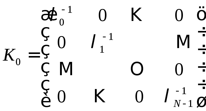
![]() –some
symmetric non-singular matrix (assumed to be known):
–some
symmetric non-singular matrix (assumed to be known):
- diagonal
– ![]() ;
;
- off the diagonal – nonzero error covariance.
Assumptions
for selection ![]() :
:
1. The linear model with heteroscedastic errors:
2. The linear model with autocorrelated errors:
![]() (correlation
coefficients of neighboring errors)
(correlation
coefficients of neighboring errors)

Note:
conventional OLS ( )remain
unbiased and consistent and OLMMR, but ineffective, that is, there
are better obtained by OLS; ordinary least squares estimation error
variance () is shifted (low), that is, giving lozhnooptimistichnye
implications for the standard errors of regression
coefficients.Обобщенный МНК
)remain
unbiased and consistent and OLMMR, but ineffective, that is, there
are better obtained by OLS; ordinary least squares estimation error
variance () is shifted (low), that is, giving lozhnooptimistichnye
implications for the standard errors of regression
coefficients.Обобщенный МНК
It is
necessary to find ![]() и
и ![]() with given z
и
with given z
и ![]() .
.
We reduce OLMMR to KLMMR.
It is known
that every symmetric nonsingular matrix A admits the representation![]() ,
where C –
some non-singular matrix. We expand
,
where C –
some non-singular matrix. We expand![]() .
.
Multiply (1) on the left C-1:
![]() .
relabel
.
relabel
![]() .
.
Minimizing![]() ,(1*)
,(1*)
As earlier
we have: ![]() and, returning to the original observations:
and, returning to the original observations:
![]() .
(1**)
.
(1**)
Let us show that, as in KLMMR:
![]()
![]()
![]() ,
so the covariance matrix of regression coefficients for OLS:
,
so the covariance matrix of regression coefficients for OLS:
![]() .
.
Nonshifted coefficient
estimate
![]() :
:
 .
.
The coefficient of determination:
 ,
not nessesary
,
not nessesary ![]() ,
have accessory, the heuristic value.
,
have accessory, the heuristic value.
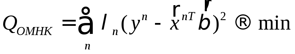
![]() ,
obtain a criterion
,
obtain a criterion
![]() (2)
(2)
the initial data OLMMR. decision know: (1**).
Note:
situations when ![]() known, are extremely rare (
known, are extremely rare (![]() ).
).
In
practically feasible GLS is necessary to introduce a priori
restrictions on the structure of the matrix ![]()
heteroscedastic errors.
Substituting
 в (2),we have
 .
(3)
.
(3)
Therefore,
OLS in this case is called the weighted least squares (![]() ).
).
(3) it
follows that for the production of ![]() more strongly influenced by the data with less error variance.
more strongly influenced by the data with less error variance.
Note: to test the hypothesis of homo / heteroscedasticity errors:
![]() (homo);
(homo);
![]() (heteroscedasticity).
(heteroscedasticity).
break the
sample {![]() }
onG
clusters (g
= 1, ..., G)
}
onG
clusters (g
= 1, ..., G)