Verification and validation of the model

Verification

- A check of conformity operation algorithm simulation model to the plan, which was laid at its development. Most often this is done considering the boundary (limit) cases (parameters) under which there is an obvious solution found, or deductively. Stochastic elements are replaced by deterministic and / or make other simplifications.

Checking the adequacy of the model

- A comparison of the simulation model with the real system that it models, ie. E. System must exist, that does not always happen.

One way to check - comparison of the expectations of the real system response Y * Y and the simulation model with the same external actions, ie. E. Tests the hypothesis:

.

Carried out a small number M of expensive experiments on a real system. obtain a sample: . Carried out a large number N of experiments on the simulation model. Obtain a sample:. Calculated significance level data , where . Such a test should be carried out for all of recorded responses.

An error estimate for the resulting indicator simulation due to the difference of seed number random number generator

Pseudo random number generators are imperfect, and using different "priming», seed number leads to different sequences of pseudorandom numbers, and hence to the various responses.

Or, if the generator is considered quite random, it is spread in the response due to the random nature of the "first impulse" (the initial conditions of the system).

In any case, the resulting error indicator simulation due to differences seed can be estimated by conducting M restarts the simulation under different seed.

Example 7.1. Let res - vector sample of the resulting indicator simulation result. Obtained at different seed ceteris paribus.

–оценка математического ожидания по выборке

–оценка стандартного отклонения по выборке

- The half-width of the confidence interval with a confidence level γ for the simulation result, accidental due to different seed. Here qt (p, N) - quantile of order p of the Student distribution with N degrees of freedom, therefore, when γ = 0.95

(95 %) confidence interval

^{< result <} .

Or other words, –error, and the final result for the result:result = ores ± Δ = 5.2 ± 1.61.

Methods of reducing the variance

antithetic method

Each time a random number r ~ U (0, 1) is calculated, its complement (1 - r), which is used for the parallel determination result. Hence, if the input variable is quite large, in a parallel calculation, it will be quite small. As a rule, this leads to the values ​​and responses that negatively correlated. Making N runs, we paired results:.– sample of,–sampleof.Obvious that Y₁ Y₂ identically distributed with Y - result a simple (non-parallel computations). We introduce the random variable.

, поэтому MYбудем искать так:

. (24)

since negative, DY₀, is less than DY, until приwith . So working with Y₀, We have the same value with the expectation, but with reduced dispersion; therefore its rating and, therefore, the error in (24) will be small.

Lowering the variance in the calculation of integrals

Suppose you want to calculate the integral ;

here – density distribution of an arbitrary random variable ξ, taking values ​​on (a, b). Further argue, as before:, где - Sample of η, where x_n sample from ξ.

Choosing different distribution , will have different , and error calculating means and I. If we take (believe f(x) > 0), so factor k must be found from the normalization condition: , that gives ; but included here the integral is unknown to us the required integral! Therefore, in practice take similar with _{But so that the normalization of all was simple and generation} of this distribution would be a simple; статистически оцененных will be small.

The use of simulation (MI) compared to the methods of estimation and the analysis of their accuracy

For a variety of applications (eg, econometrics) researchers propose more and more new models and methods. Sometimes analyzed analytically (deductively) the characteristics of accuracy and predictive power of these methods can be difficult. And here comes to their aid.

Example 8.1. Required to estimate a regression function yr = β0 + β1x. Data (observations) are of the form: Yn = β0 + β1xn + En, where En - random error (feature) n-th observation. We assume En i.i.d. N (0, o).

Suppose an experiment is active, ie. E. Values ​​xn factors researchers can choose yourself.

Suppose there are two researchers. Both are going to evaluate the vector of regression coefficients least squares (OLS):

, (25)

_где , , .

The first researcher believes that the values ​​of xn factor (design matrix z) can be chosen arbitrarily, the second is surmised that the values ​​of xn is better to take orthogonal to the column of units

So . , or ^{That allegedly give "more accurate" evaluation .}

How to check if someone is better?

Idea MI: laid-known true parameters β0 and β1, N generated errors are the same for both methods, and the formula Yn = β0 + β1xn + En calculated for each researcher resulting values​​, ..., N values ​​for factor selected from them differently. Then, the two sets are estimated by (25), and it is clear that gives closer to the truth of (better)!

To "collect statistics" spend M runs:

–the number of runs,

,

To "collect statistics" spend M runs:

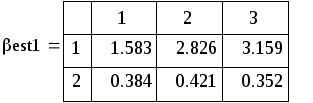
Since each run gives independent implementation of the random variable Best, the average over all the joists gives nonshifted and wealthy (in M) estimate of the expectation of Best, and Stdev () provides a consistent and asymptotically nonshifted estimate of the standard deviation Best. In particular, the estimation of the angular rate (which, as we know β1 = 0.5):

It can be seen that the second method gives closer to the truth (0.5) results (with less dispersion). In this comparison of data supposedly theoretically investigated methods can be considered complete.

Knowing the theory, we can now confirm it:

1 Increasing M, we see that the expectation of the coefficient estimates in both methods is 0.5, ie. E. They give nonshifted evaluation.

2 By increasing M, we see that the estimate of the coefficient s about u (found at M = 1000).Теория даёт:

: which is equivalent to the latter

Literature

1. Емельянов А. А. Имитационное моделирование экономических процессов : учеб. пособие для студентов, обучающихся по специальности «Прикладная информатика» / А. А. Емельянов, Е. А. Власова, Р. В. Дума ; под ред.

2. А. А. Емельянова. – М. : Финансы и статистика, 2004.

3. Лоу А. М. Имитационное моделирование / А. М. Лоу, В. Д. Кельтон ; перевод с англ. А. Куленко под ред. В. Томашевского. – 3-е изд. – М. ; СПб. ; Нижний Новгород [и др.] : Питер, 2004.

4. Советов Б. Я. Моделирование систем : учеб. для вузов / Б. Я. Советов,

5. С. А. Яковлев. – 3-е изд., перераб. и доп. – М. : Высш. шк., 2001.

Additional literature

1. Максимей И. В. Имитационное моделирование на ЭВМ / И. В. Максимей. – М. : Радио и связь, 1988.

2. Лукасевич И. Я. Анализ финансовых операций / И. Я. Лукасевич. – М. : ЮНИТИ, 1998.

3. Ивченко Г. И. Математическая статистика / Г. И. Ивченко, Ю. И. Медведев. – М. : Высш. шк., 1984.

4. Большев Л.Н.Таблицы математической статистики /Л.Н.Большев,

5. Н.В. Смирнов. – М.:Наука,1983.

6. Исследование операций в экономике / ред. Кремер Н. Ш. / М. : ЮНИТИ, 1997.

7. Айвазян С. А. Прикладная статистика и основы эконометрики /

8. С. А. Айвазян, В. С. Мхитарян. – М. : ЮНИТИ, 1998.

9. Харин Ю. С. Основы имитационного и статистического моделирования /

10. Ю. С. Харин, В. И. Малюгин, В. П. Кирлица и др. – Минск : Дизайн ПРО, 1997.

11. Уотшем Т. Дж. Количественные методы в финансах / Т. Дж. Уотшем,

12. К. Паррамоу. – М. : ЮНИТИ, 1999.

13. Плис А. И. Mathcad2000. Математический практикум для экономистов и инженеров : учеб. пособие / А. И. Плис, Н. А. Сливина.– М. : Финансы и статистика, 2000.

14. Клейнен Дж. Статистические методы в имитационном моделировании :

15. в 2 т. [пер. с англ.]. / Дж. Клейнен. – Серия: Математико-статистические методы за рубежом. – М. : Статистика, 1978.

16. Коршунов Ю. М. Математические основы кибернетики / Ю. М. Коршунов. – М. : Энергоатомиздат, 1987.

17. Справочник по прикладной статистике: в 2 т. / Ред.Э.Ллойд,У.Ледерман.– М.:Финансы и статистика,1990.

18. Соболь И. М. Метод Монте-Карло / И. М. Соболь. – М. : Наука, 1972.

19. Кофман А. Займёмся исследованием операций / А. Кофман, Р. Фор. – М. : Мир, 1966.

20. Чистяков В. П. Курс теории вероятностей / В. П. Чистяков. – М. : Наука, 1982.

21. Пакет программ GPSS. Режим доступа:

22. http://www.minutemansoftware.com/downloads/student.exe

23. Кудрявцев Е. М. GPSS World. Основы имитационного моделирования различных систем / Е. М. Кудрявцев. – М. : ДМК Пресс, 2004.

24. Бородачёв С. М.Элементы математической статистики. Режим доступа: http://study.ustu.ru/view/aid_view.aspx?AidId=372