

Лаб.7
.docxЛабораторная работа №7 “Метод Эйлера. Схема Рунге-Кутта решения ОДУ”
Теория:
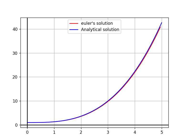
from typing import Union from numpy import linspace import matplotlib.pyplot as plt def euler(f: callable, start_point: tuple[Union[int, float], Union[int, float]], end: Union[int, float], n: int = 50) \ -> tuple[tuple[float], list[float]]: """ :param f: Function to solve f(x,y) :param start_point: Tuple of (x,y) as initial condition :param end: end x :param n: number of points :return: (X:tuple,Y:tuple) """ h = abs(start_point[0] - end) / n x = tuple(start_point[0] + i * h for i in range(n)) y = [start_point[1]] for i in range(1, len(x)): y.append(y[i - 1] + h * f(x[i - 1], y[i - 1])) return x, y if __name__ == '__main__': f = lambda x, y: x ** 2 ex, ey = euler(f, (0, 1), 5, 100) x = linspace(0, 5) y = tuple(i ** 3 / 3 + 1 for i in x) diff = max(abs(ey[i] - (ex[i] ** 3 / 3 + 1)) for i in range(len(ex))) print(f'Max difference between euler and analytical is {diff}') plt.plot(ex, ey, 'r', label="euler's solution") plt.plot(x, y, 'b', label='Analytical solution') plt.axhline(color='k') plt.axvline(color='k') plt.legend() plt.grid() plt.show()
Функция:
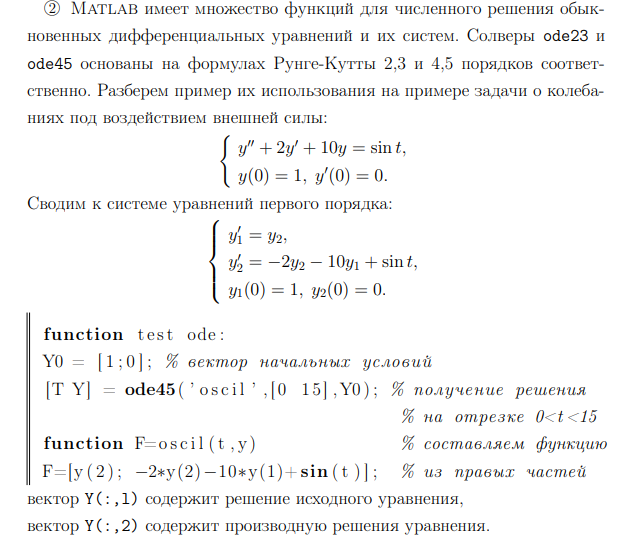
function [ dydt ] = solver( t,Y0 )
dydt=[Y0(2) ; -2*Y0(2)-10*Y0(1)+ sin(t) ] ;
end
Код Матлаб:
Y0 = [1;0] ;
[t1 y1] = ode23( @solver, [0 15] ,Y0 );
[t2 y2] = ode45( @solver, [0 15] ,Y0 );
subplot(2,3,1)
plot(t1,y1(:,1))
axis([0 15 -0.5 1])
legend('y1')
title('ode23')
grid on
subplot(2,3,2)
plot(t2,y2(:,1))
axis([0 15 -0.5 1])
grid on
legend('y1')
title('ode45')
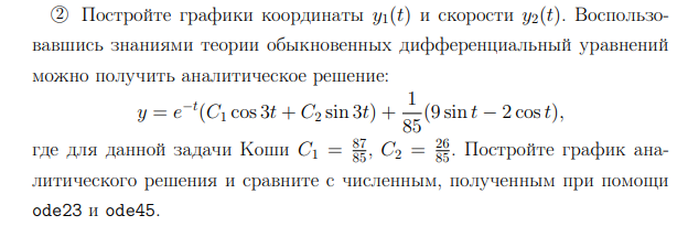
c1=87/85;
c2=26/85;
f=@(t)exp(-t)*(c1*cos(3*t)+c2*sin(3*t))+1/85*(9*sin(t)-2*cos(t));
df=@(t)exp(-t)*(-3*c1*sin(3*t)+3*c2*cos(3*t))-exp(-t)*(c1*cos(3*t)+c2*sin(3*t))+1/85*(9*cos(t)+2*sin(t));
subplot(2,3,3)
fplot(f,[0 15])
grid on
legend('y1')
title('solve')
subplot(2,3,4)
plot(t1,y1(:,2))
axis([0 15 -3 1])
legend('y2')
title('ode23')
grid on
subplot(2,3,5)
plot(t2,y2(:,2))
axis([0 15 -3 1])
legend('y2')
title('ode45')
grid on
subplot(2,3,6)
fplot(df,[0 15])
legend('y2')
title('solve')
grid on
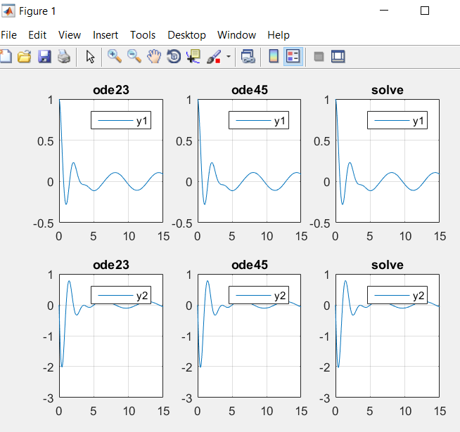
Верхняя строка зависимость координаты от времени 3 график является точным решением диффура второго порядка. Нижняя строка зависимость скорости от времени 6 график является производной точного решения диффура второго порядка. Численные решения с большой точностью совпадают с истинным решением.
Функция:
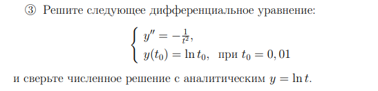
function [ dydt ] = solver2_( t,Y0 )
dydt=[Y0(2) ; -1/t^2 ] ;
end
Код Матлаб:
hold on
grid on
Y0 = [ log(0.01) ; 1/0.01 ] ;
[t y] = ode45( @solver2_, [0.01 1] ,Y0 );
plot(t,y(:,1))
fplot(@(t) log(t),[0.01 1],'r')
xlabel('t')
ylabel('y')
title('d2y=-1/t^2, y(0.01)=ln(0.01)')
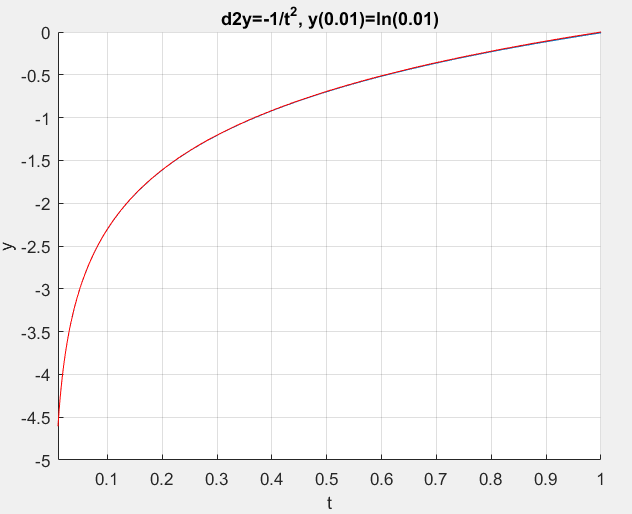
Синей кривой отмечено численное решение диффура, красной кривой точное решение. Как видно они почти сливаются, а значит решение верно.