10.1  BASIC PRINCIPLE AND IMPLEMENTATION OF WAVE FIELD SYNTHESIS

440  Spatial Sound

boundary surface (or curve) and then reproduced by the corresponding secondary source array. This principle is the basic concept of wavefront reproduction technique and system.

At the early stage of spatial sound, a primitive technique based on the Huygens–Fresnel principle was proposed for sound field recording and reproduction. For instance, in the work at Bell Labs in the 1930s, an “acoustic curtain” (array in vertical plane) of pressure (omnidirectional) microphones in front of a stage was suggested for recording wavefronts; the signals were then reproduced through a loudspeaker array with the same configuration as that of the microphone array on the receiver side (Steinberg and Snow, 1934; Snow, 1953). Through the simplification of the “acoustic curtain,” twoand three-channel-spaced microphone techniques have been developed, as described in Section 2.2.3. After simplification, the reproduced sound field is greatly different from the sound recorded and reproduced by an “acoustic curtain.” Olson (1969) also recommended using 15 microphones arranged in a close horizontal curve to record the sound field and then reproduce signals with the corresponding loudspeaker configuration. Of the total number of microphones, seven are frontal microphones for recording the direct sound from the stage, and eight are lateral and rear microphones for recording the reflections of halls.

These previous studies only suggested the conceptual method of recording and reconstructing the wavefront of a sound field without strict mathematical and physical justification. They also did not derive the required radiation characteristics and driving signals of secondary sources. Since 1988, Berkhout (1988), Berkhout et al. (1993) and the group at Delft University of Technology have conducted a series of pioneering works on wavefront reconstruction (Boone et al., 1995; Vries, 1996, 2009). The technique and principle of WFS were developed on the basis of the principle of acoustical holography (Williams, 1999), and the radiation characteristics and driving signals of secondary sources were derived. Since the 1990s, WFS has been recognized as an interesting topic in spatial sound technique. As a part of the research on creating interactive audiovisual environments, numerous works on WFS under the framework project of EC IST CARROUSO have been conducted by European groups (Brix et al., 2001). Since then, theory of WFS has been greatly improved (Spors et al., 2008; Ahrens 2012).

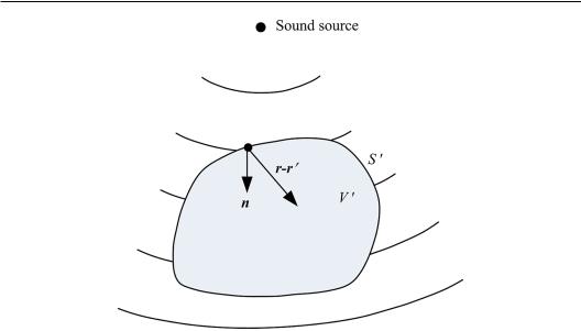
Mathematically, the Huygens–Fresnel principle is described by Kirchhoff–Helmholtz boundary integral equation. As illustrated in Figure 10.1, the frequency-dependent sound pressure P(r, f) in an arbitrary source-free and closed space V′ is determined by the pressure and its normal derivative on the boundary surface S′ of V′:

S

where f is the frequency; r and r′ are the vector of the receiver position inside V′ and the vector of a point on the boundary surface S′, respectively; and ∂/∂n′ is an inward-normal derivative on the surface of S′. The integral is calculated over the entire boundary surface S′. Gfree3D r, r , f is free-field Green’s function in a three-dimensional space (and frequency domain) expressed in Equation (9.2.2), which represents the sound pressure at the receiver position r caused by a monopole point source at position r′ with the unit strength

Spatial sound reproduction by wave field synthesis 441

Figure 10.1 Sketch of Kirchhoff–Helmholtz integral.

In Equation (10.1.1), the normal derivative of Green’s function is calculated by

where n′ is a unit vector in the inward-normal direction at r′ on S′; and (r – r′)/| r – r′ | is a unit vector pointing from r′ to r. Equation (10.1.3) describes the sound pressure at r caused by a dipole source with unit strength and at r′, with the main axis of the dipole source pointing to the n′ direction. θr n is the angle between vectors (r – r′) and n′.

According to Equation (3.2.11), ∂P(r′,f )/∂n′ is directly proportional to the medium velocity component in the inward-normal direction of surface S′:

Equation (10.1.1) and the discussion above indicate that the closed boundary surface can be equivalent to the continuous distribution of two types of secondary sources, i.e., monopole (point) and dipole secondary sources on the surface. The strength of monopole secondary sources is directly proportional to the derivative of pressure in the outward-normal direction (or an equally medium velocity component in the inward-normal direction) of S′. The strength of the dipole secondary source is directly proportional to the pressure on the surface S′. Therefore, the pressures and medium velocity on a closed surface S′ in the original sound fields can be captured by uniform and continuous arrays of pressure (omnidirectional) and velocity field (bidirectional) microphones, respectively. The outputs of these two microphone

442  Spatial Sound

arrays are used as driving signals of the corresponding dipole and monopole secondary source arrays arranged on the closed boundary surface of the receiver space to reconstruct the target sound field. As stated in Section 1.2.5, however, practical velocity field microphones are designed so that their magnitude responses are independent of the frequency of a far-field incident plane wave. These velocity field microphones cannot be used directly to capture the medium velocity on the boundary surface. In practice, the pressure and its inward-normal derivative on a boundary surface in the original sound field can also be evaluated through calculation and simulation, and the microphone array for recording in the original sound field is unnecessary. This description is the basic principle of sound reproduction via an acoustical holographic technique. Some terms used in this chapter should be explained. The acoustical holographic technique or acoustical holography usually refers to techniques and systems based on accurate Kirchhoff–Helmholtz boundary integral and accurate sound field reconstruction. From the point of practical uses, the results of Kirchhoff–Helmholtz boundary integral should be simplified. WFS usually refers to a specified technique and system based on an approximation of the Kirchhoff–Helmholtz boundary integral. As in the case of Chapter 9, when acoustical holography and WFS are analyzed, the terms secondary source and driving signals are used.

The following problems should be considered to transform from ideal acoustical holography to practical WFS.

1. Simplification of the types of secondary sources

A complete acoustical holography requires two types of secondary sources with different radiation characteristics, e.g., monopole and dipole sources. In practice, one type of secondary sources alone is preferred. Therefore, the types of secondary sources should be simplified.

2. Simplification of spatial dimensionality in reproduction

Sound information reproduction in a three-dimensional space requires a three-dimen- sional secondary source array arranged on the closed boundary surface S′ of volume V′ and thus requires a large number of secondary sources. Numerous secondary sources are usually impractical. Moreover, secondary sources arranged on a closed surface are often in conflict with visual requirements of many practical applications. In this case, spatial dimensionality in reproduction should be reduced to simplify the secondary source array.

3Discrete and finite secondary source array

An ideal WFS requires a continuous array with an infinite number of secondary sources. However, a discrete and finite array of secondary sources is available in practical WFS. This discrete array leads to a spatial aliasing error, and a finite array causes an edge diffraction effect in the reconstructed sound field.

These problems are addressed in Sections 10.1.2 to 10.1.5 from the point of the practical implementation of WFS.

10.1.2  Simplification of the types of secondary sources

According to Equation (10.1.1), acoustical holography requires secondary source arrays of monopole and dipole types. The system can be simplified when an array of either monopole or dipole secondary sources is enough to reconstruct the target sound field. As illustrated in Figure 10.2, a target (primary) source is located on one (the left) side of an infinite (vertical) plane S′1. A source-free half-space V′ of the receiver is located on another side (right side) of the plane S′1. The plane S′1 and the hemispherical surface S′2 with an infinite radius on the