24 Spatial Sound

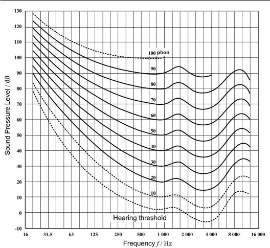
Figure 1.12 Normal equal-loudness level contours by the ISO (plane wave incidence from the front, pure tone, and binaural listening; adapted from ISO 226, 2003).

4. The contours flatten for high SPL or loudness levels, reducing the differences in the loudness of different frequencies at a constant high SPL.

The normal equal-loudness level contours by the ISO are the statistical results on young subjects with normal hearing. They represent the regular pattern of human loudness perception. Some (or even considerable) differences may exist between the ISO contours and those of each individual.

The results of some psychoacoustic experiments indicate that loudness depends on the incident direction of a plane wave (or sound source direction) for a free-field plane wave with a given frequency and SPL. This finding is the directional loudness in the free field. Directional loudness is an issue related to binaural hearing (Sivonen and Ellermeier, 2008; Moore and Glasberg, 2007; Section 1.6.5).

1.3.3 Masking

Masking refers to the psychoacoustic phenomenon in which the auditory detection threshold of a sound (target) may increase in the presence of another sound (masker). The masking threshold is the minimum SPL of a target that is detectable in the presence of a masker. The

Sound field, spatial hearing, and sound reproduction  25

amount of masking is the difference in the detectable thresholds of the SPL between the presence and absence of the masker.

The masking threshold and amount of masking vary with multiple factors, including the types, strength, frequency spectrum, temporal relationship, and spatial positions of targets and maskers. Given the types, temporal relationship, and spatial positions of targets and maskers, the masking threshold or amount of masking at various target frequencies and for different SPL and frequencies of a masker can be determined via psychoacoustic measurements. As a result, a series of masking curves or patterns is formed. Masking patterns depend on the type of targets and maskers. The results of a tone masked by another tone and a tone masked by another band-pass noise are common. Two experimental methods are utilized to measure the masking. Accordingly, the SPL is determined at two different reference positions. One is to measure the monaural or binaural masking via headphone presentation, and the SPL is determined at a certain position in the external ear (e.g., the entrance of the ear canal or eardrum). The other is to measure the masking of a free-field target and a masker, and the SPL is identified at the position of head center in the absence of the head. The SPLs measured from two reference positions are different because of the scattering and diffraction effects of the head and pinna when a subject enters the sound field. However, they can be converted to each other by using head-related transfer functions (Section 1.4.2).

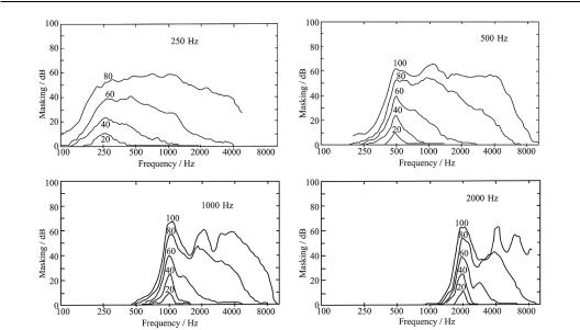
Figure 1.13 illustrates the monoaural masking patterns of a tone by another tone (Ehmer, 1959a, 1959b), and these patterns represent the amount of masking as a function of the target frequency at various SPLs of a tone masker. The target sound and masker are presented simultaneously, i.e., the case of simultaneous masking.

Figure 1.13 presents the following:

1. Masking is effective when the frequency spectra of a masker and a target are close to each other.

2. Masking patterns are asymmetric. More masking occurs for the target frequency that is higher than the masker frequency, and less masking occurs for the target frequency that is lower than the masker frequency.

3. As the SPL of the masker increases, the range covered by masking widens, especially toward a high frequency range.

Masking occurs when a masker and a target are presented successively. This phenomenon is called temporal or nonsimultaneous masking. Temporal masking is subdivided into backward masking (premasking) and forward masking (postmasking). For backward masking, the target is presented prior to the masker. For forward masking, the target is presented after the masker. The durations of forward and backward masking are different. Generally, forward masking lasts 200 ms, and backward masking only lasts 15–20 ms. However, the mechanism of temporal masking is still unclear.

The masking threshold or amount of masking for a spatially separated masker and target is lower than that for a spatially coincident masker and target. Spatial unmasking is the phenomenon that the spatial separation of the masker and target – in terms of direction and distance – decreases the masking threshold or the amount of masking (Kopčo and ShinnCunningham, 2003). It is a binaural phenomenon associated with head-related transfer functions and spatial cues in binaural pressures (Section 1.6.5).

1.3.4  Critical band and auditory filter

Fletcher (1940) investigated the masking of a tone by a band-pass noise and reported that noise in a bandwidth centered at the tone frequency is effective in masking the tone. Conversely, the other noise component outside the bandwidth has no effect on masking.