
- •Preface
- •Introduction
- •1.1 Spatial coordinate systems
- •1.2 Sound fields and their physical characteristics
- •1.2.1 Free-field and sound waves generated by simple sound sources
- •1.2.2 Reflections from boundaries
- •1.2.3 Directivity of sound source radiation
- •1.2.4 Statistical analysis of acoustics in an enclosed space
- •1.2.5 Principle of sound receivers
- •1.3 Auditory system and perception
- •1.3.1 Auditory system and its functions
- •1.3.2 Hearing threshold and loudness
- •1.3.3 Masking
- •1.3.4 Critical band and auditory filter
- •1.4 Artificial head models and binaural signals
- •1.4.1 Artificial head models
- •1.4.2 Binaural signals and head-related transfer functions
- •1.5 Outline of spatial hearing
- •1.6 Localization cues for a single sound source
- •1.6.1 Interaural time difference
- •1.6.2 Interaural level difference
- •1.6.3 Cone of confusion and head movement
- •1.6.4 Spectral cues
- •1.6.5 Discussion on directional localization cues
- •1.6.6 Auditory distance perception
- •1.7 Summing localization and spatial hearing with multiple sources
- •1.7.1 Summing localization with two sound sources
- •1.7.2 The precedence effect
- •1.7.3 Spatial auditory perceptions with partially correlated and uncorrelated source signals
- •1.7.4 Auditory scene analysis and spatial hearing
- •1.7.5 Cocktail party effect
- •1.8 Room reflections and auditory spatial impression
- •1.8.1 Auditory spatial impression
- •1.8.2 Sound field-related measures and auditory spatial impression
- •1.8.3 Binaural-related measures and auditory spatial impression
- •1.9.1 Basic principle of spatial sound
- •1.9.2 Classification of spatial sound
- •1.9.3 Developments and applications of spatial sound
- •1.10 Summary
- •2.1 Basic principle of a two-channel stereophonic sound
- •2.1.1 Interchannel level difference and summing localization equation
- •2.1.2 Effect of frequency
- •2.1.3 Effect of interchannel phase difference
- •2.1.4 Virtual source created by interchannel time difference
- •2.1.5 Limitation of two-channel stereophonic sound
- •2.2.1 XY microphone pair
- •2.2.2 MS transformation and the MS microphone pair
- •2.2.3 Spaced microphone technique
- •2.2.4 Near-coincident microphone technique
- •2.2.5 Spot microphone and pan-pot technique
- •2.2.6 Discussion on microphone and signal simulation techniques for two-channel stereophonic sound
- •2.3 Upmixing and downmixing between two-channel stereophonic and mono signals
- •2.4 Two-channel stereophonic reproduction
- •2.4.1 Standard loudspeaker configuration of two-channel stereophonic sound
- •2.4.2 Influence of front-back deviation of the head
- •2.5 Summary
- •3.1 Physical and psychoacoustic principles of multichannel surround sound
- •3.2 Summing localization in multichannel horizontal surround sound
- •3.2.1 Summing localization equations for multiple horizontal loudspeakers
- •3.2.2 Analysis of the velocity and energy localization vectors of the superposed sound field
- •3.2.3 Discussion on horizontal summing localization equations
- •3.3 Multiple loudspeakers with partly correlated and low-correlated signals
- •3.4 Summary
- •4.1 Discrete quadraphone
- •4.1.1 Outline of the quadraphone
- •4.1.2 Discrete quadraphone with pair-wise amplitude panning
- •4.1.3 Discrete quadraphone with the first-order sound field signal mixing
- •4.1.4 Some discussions on discrete quadraphones
- •4.2 Other horizontal surround sounds with regular loudspeaker configurations
- •4.2.1 Six-channel reproduction with pair-wise amplitude panning
- •4.2.2 The first-order sound field signal mixing and reproduction with M ≥ 3 loudspeakers
- •4.3 Transformation of horizontal sound field signals and Ambisonics
- •4.3.1 Transformation of the first-order horizontal sound field signals
- •4.3.2 The first-order horizontal Ambisonics
- •4.3.3 The higher-order horizontal Ambisonics
- •4.3.4 Discussion and implementation of the horizontal Ambisonics
- •4.4 Summary
- •5.1 Outline of surround sounds with accompanying picture and general uses
- •5.2 5.1-Channel surround sound and its signal mixing analysis
- •5.2.1 Outline of 5.1-channel surround sound
- •5.2.2 Pair-wise amplitude panning for 5.1-channel surround sound
- •5.2.3 Global Ambisonic-like signal mixing for 5.1-channel sound
- •5.2.4 Optimization of three frontal loudspeaker signals and local Ambisonic-like signal mixing
- •5.2.5 Time panning for 5.1-channel surround sound
- •5.3 Other multichannel horizontal surround sounds
- •5.4 Low-frequency effect channel
- •5.5 Summary
- •6.1 Summing localization in multichannel spatial surround sound
- •6.1.1 Summing localization equations for spatial multiple loudspeaker configurations
- •6.1.2 Velocity and energy localization vector analysis for multichannel spatial surround sound
- •6.1.3 Discussion on spatial summing localization equations
- •6.1.4 Relationship with the horizontal summing localization equations
- •6.2 Signal mixing methods for a pair of vertical loudspeakers in the median and sagittal plane
- •6.3 Vector base amplitude panning
- •6.4 Spatial Ambisonic signal mixing and reproduction
- •6.4.1 Principle of spatial Ambisonics
- •6.4.2 Some examples of the first-order spatial Ambisonics
- •6.4.4 Recreating a top virtual source with a horizontal loudspeaker arrangement and Ambisonic signal mixing
- •6.5 Advanced multichannel spatial surround sounds and problems
- •6.5.1 Some advanced multichannel spatial surround sound techniques and systems
- •6.5.2 Object-based spatial sound
- •6.5.3 Some problems related to multichannel spatial surround sound
- •6.6 Summary
- •7.1 Basic considerations on the microphone and signal simulation techniques for multichannel sounds
- •7.2 Microphone techniques for 5.1-channel sound recording
- •7.2.1 Outline of microphone techniques for 5.1-channel sound recording
- •7.2.2 Main microphone techniques for 5.1-channel sound recording
- •7.2.3 Microphone techniques for the recording of three frontal channels
- •7.2.4 Microphone techniques for ambience recording and combination with frontal localization information recording
- •7.2.5 Stereophonic plus center channel recording
- •7.3 Microphone techniques for other multichannel sounds
- •7.3.1 Microphone techniques for other discrete multichannel sounds
- •7.3.2 Microphone techniques for Ambisonic recording
- •7.4 Simulation of localization signals for multichannel sounds
- •7.4.1 Methods of the simulation of directional localization signals
- •7.4.2 Simulation of virtual source distance and extension
- •7.4.3 Simulation of a moving virtual source
- •7.5 Simulation of reflections for stereophonic and multichannel sounds
- •7.5.1 Delay algorithms and discrete reflection simulation
- •7.5.2 IIR filter algorithm of late reverberation
- •7.5.3 FIR, hybrid FIR, and recursive filter algorithms of late reverberation
- •7.5.4 Algorithms of audio signal decorrelation
- •7.5.5 Simulation of room reflections based on physical measurement and calculation
- •7.6 Directional audio coding and multichannel sound signal synthesis
- •7.7 Summary
- •8.1 Matrix surround sound
- •8.1.1 Matrix quadraphone
- •8.1.2 Dolby Surround system
- •8.1.3 Dolby Pro-Logic decoding technique
- •8.1.4 Some developments on matrix surround sound and logic decoding techniques
- •8.2 Downmixing of multichannel sound signals
- •8.3 Upmixing of multichannel sound signals
- •8.3.1 Some considerations in upmixing
- •8.3.2 Simple upmixing methods for front-channel signals
- •8.3.3 Simple methods for Ambient component separation
- •8.3.4 Model and statistical characteristics of two-channel stereophonic signals
- •8.3.5 A scale-signal-based algorithm for upmixing
- •8.3.6 Upmixing algorithm based on principal component analysis
- •8.3.7 Algorithm based on the least mean square error for upmixing
- •8.3.8 Adaptive normalized algorithm based on the least mean square for upmixing
- •8.3.9 Some advanced upmixing algorithms
- •8.4 Summary
- •9.1 Each order approximation of ideal reproduction and Ambisonics
- •9.1.1 Each order approximation of ideal horizontal reproduction
- •9.1.2 Each order approximation of ideal three-dimensional reproduction
- •9.2 General formulation of multichannel sound field reconstruction
- •9.2.1 General formulation of multichannel sound field reconstruction in the spatial domain
- •9.2.2 Formulation of spatial-spectral domain analysis of circular secondary source array
- •9.2.3 Formulation of spatial-spectral domain analysis for a secondary source array on spherical surface
- •9.3 Spatial-spectral domain analysis and driving signals of Ambisonics
- •9.3.1 Reconstructed sound field of horizontal Ambisonics
- •9.3.2 Reconstructed sound field of spatial Ambisonics
- •9.3.3 Mixed-order Ambisonics
- •9.3.4 Near-field compensated higher-order Ambisonics
- •9.3.5 Ambisonic encoding of complex source information
- •9.3.6 Some special applications of spatial-spectral domain analysis of Ambisonics
- •9.4 Some problems related to Ambisonics
- •9.4.1 Secondary source array and stability of Ambisonics
- •9.4.2 Spatial transformation of Ambisonic sound field
- •9.5 Error analysis of Ambisonic-reconstructed sound field
- •9.5.1 Integral error of Ambisonic-reconstructed wavefront
- •9.5.2 Discrete secondary source array and spatial-spectral aliasing error in Ambisonics
- •9.6 Multichannel reconstructed sound field analysis in the spatial domain
- •9.6.1 Basic method for analysis in the spatial domain
- •9.6.2 Minimizing error in reconstructed sound field and summing localization equation
- •9.6.3 Multiple receiver position matching method and its relation to the mode-matching method
- •9.7 Listening room reflection compensation in multichannel sound reproduction
- •9.8 Microphone array for multichannel sound field signal recording
- •9.8.1 Circular microphone array for horizontal Ambisonic recording
- •9.8.2 Spherical microphone array for spatial Ambisonic recording
- •9.8.3 Discussion on microphone array recording
- •9.9 Summary
- •10.1 Basic principle and implementation of wave field synthesis
- •10.1.1 Kirchhoff–Helmholtz boundary integral and WFS
- •10.1.2 Simplification of the types of secondary sources
- •10.1.3 WFS in a horizontal plane with a linear array of secondary sources
- •10.1.4 Finite secondary source array and effect of spatial truncation
- •10.1.5 Discrete secondary source array and spatial aliasing
- •10.1.6 Some issues and related problems on WFS implementation
- •10.2 General theory of WFS
- •10.2.1 Green’s function of Helmholtz equation
- •10.2.2 General theory of three-dimensional WFS
- •10.2.3 General theory of two-dimensional WFS
- •10.2.4 Focused source in WFS
- •10.3 Analysis of WFS in the spatial-spectral domain
- •10.3.1 General formulation and analysis of WFS in the spatial-spectral domain
- •10.3.2 Analysis of the spatial aliasing in WFS
- •10.3.3 Spatial-spectral division method of WFS
- •10.4 Further discussion on sound field reconstruction
- •10.4.1 Comparison among various methods of sound field reconstruction
- •10.4.2 Further analysis of the relationship between acoustical holography and sound field reconstruction
- •10.4.3 Further analysis of the relationship between acoustical holography and Ambisonics
- •10.4.4 Comparison between WFS and Ambisonics
- •10.5 Equalization of WFS under nonideal conditions
- •10.6 Summary
- •11.1 Basic principles of binaural reproduction and virtual auditory display
- •11.1.1 Binaural recording and reproduction
- •11.1.2 Virtual auditory display
- •11.2 Acquisition of HRTFs
- •11.2.1 HRTF measurement
- •11.2.2 HRTF calculation
- •11.2.3 HRTF customization
- •11.3 Basic physical features of HRTFs
- •11.3.1 Time-domain features of far-field HRIRs
- •11.3.2 Frequency domain features of far-field HRTFs
- •11.3.3 Features of near-field HRTFs
- •11.4 HRTF-based filters for binaural synthesis
- •11.5 Spatial interpolation and decomposition of HRTFs
- •11.5.1 Directional interpolation of HRTFs
- •11.5.2 Spatial basis function decomposition and spatial sampling theorem of HRTFs
- •11.5.3 HRTF spatial interpolation and signal mixing for multichannel sound
- •11.5.4 Spectral shape basis function decomposition of HRTFs
- •11.6 Simplification of signal processing for binaural synthesis
- •11.6.1 Virtual loudspeaker-based algorithms
- •11.6.2 Basis function decomposition-based algorithms
- •11.7.1 Principle of headphone equalization
- •11.7.2 Some problems with binaural reproduction and VAD
- •11.8 Binaural reproduction through loudspeakers
- •11.8.1 Basic principle of binaural reproduction through loudspeakers
- •11.8.2 Virtual source distribution in two-front loudspeaker reproduction
- •11.8.3 Head movement and stability of virtual sources in Transaural reproduction
- •11.8.4 Timbre coloration and equalization in transaural reproduction
- •11.9 Virtual reproduction of stereophonic and multichannel surround sound
- •11.9.1 Binaural reproduction of stereophonic and multichannel sound through headphones
- •11.9.2 Stereophonic expansion and enhancement
- •11.9.3 Virtual reproduction of multichannel sound through loudspeakers
- •11.10.1 Binaural room modeling
- •11.10.2 Dynamic virtual auditory environments system
- •11.11 Summary
- •12.1 Physical analysis of binaural pressures in summing virtual source and auditory events
- •12.1.1 Evaluation of binaural pressures and localization cues
- •12.1.2 Method for summing localization analysis
- •12.1.3 Binaural pressure analysis of stereophonic and multichannel sound with amplitude panning
- •12.1.4 Analysis of summing localization with interchannel time difference
- •12.1.5 Analysis of summing localization at the off-central listening position
- •12.1.6 Analysis of interchannel correlation and spatial auditory sensations
- •12.2 Binaural auditory models and analysis of spatial sound reproduction
- •12.2.1 Analysis of lateral localization by using auditory models
- •12.2.2 Analysis of front-back and vertical localization by using a binaural auditory model
- •12.2.3 Binaural loudness models and analysis of the timbre of spatial sound reproduction
- •12.3 Binaural measurement system for assessing spatial sound reproduction
- •12.4 Summary
- •13.1 Analog audio storage and transmission
- •13.1.1 45°/45° Disk recording system
- •13.1.2 Analog magnetic tape audio recorder
- •13.1.3 Analog stereo broadcasting
- •13.2 Basic concepts of digital audio storage and transmission
- •13.3 Quantization noise and shaping
- •13.3.1 Signal-to-quantization noise ratio
- •13.3.2 Quantization noise shaping and 1-Bit DSD coding
- •13.4 Basic principle of digital audio compression and coding
- •13.4.1 Outline of digital audio compression and coding
- •13.4.2 Adaptive differential pulse-code modulation
- •13.4.3 Perceptual audio coding in the time-frequency domain
- •13.4.4 Vector quantization
- •13.4.5 Spatial audio coding
- •13.4.6 Spectral band replication
- •13.4.7 Entropy coding
- •13.4.8 Object-based audio coding
- •13.5 MPEG series of audio coding techniques and standards
- •13.5.1 MPEG-1 audio coding technique
- •13.5.2 MPEG-2 BC audio coding
- •13.5.3 MPEG-2 advanced audio coding
- •13.5.4 MPEG-4 audio coding
- •13.5.5 MPEG parametric coding of multichannel sound and unified speech and audio coding
- •13.5.6 MPEG-H 3D audio
- •13.6 Dolby series of coding techniques
- •13.6.1 Dolby digital coding technique
- •13.6.2 Some advanced Dolby coding techniques
- •13.7 DTS series of coding technique
- •13.8 MLP lossless coding technique
- •13.9 ATRAC technique
- •13.10 Audio video coding standard
- •13.11 Optical disks for audio storage
- •13.11.1 Structure, principle, and classification of optical disks
- •13.11.2 CD family and its audio formats
- •13.11.3 DVD family and its audio formats
- •13.11.4 SACD and its audio formats
- •13.11.5 BD and its audio formats
- •13.12 Digital radio and television broadcasting
- •13.12.1 Outline of digital radio and television broadcasting
- •13.12.2 Eureka-147 digital audio broadcasting
- •13.12.3 Digital radio mondiale
- •13.12.4 In-band on-channel digital audio broadcasting
- •13.12.5 Audio for digital television
- •13.13 Audio storage and transmission by personal computer
- •13.14 Summary
- •14.1 Outline of acoustic conditions and requirements for spatial sound intended for domestic reproduction
- •14.2 Acoustic consideration and design of listening rooms
- •14.3 Arrangement and characteristics of loudspeakers
- •14.3.1 Arrangement of the main loudspeakers in listening rooms
- •14.3.2 Characteristics of the main loudspeakers
- •14.3.3 Bass management and arrangement of subwoofers
- •14.4 Signal and listening level alignment
- •14.5 Standards and guidance for conditions of spatial sound reproduction
- •14.6 Headphones and binaural monitors of spatial sound reproduction
- •14.7 Acoustic conditions for cinema sound reproduction and monitoring
- •14.8 Summary
- •15.1 Outline of psychoacoustic and subjective assessment experiments
- •15.2 Contents and attributes for spatial sound assessment
- •15.3 Auditory comparison and discrimination experiment
- •15.3.1 Paradigms of auditory comparison and discrimination experiment
- •15.3.2 Examples of auditory comparison and discrimination experiment
- •15.4 Subjective assessment of small impairments in spatial sound systems
- •15.5 Subjective assessment of a spatial sound system with intermediate quality
- •15.6 Virtual source localization experiment
- •15.6.1 Basic methods for virtual source localization experiments
- •15.6.2 Preliminary analysis of the results of virtual source localization experiments
- •15.6.3 Some results of virtual source localization experiments
- •15.7 Summary
- •16.1.1 Application to commercial cinema and related problems
- •16.1.2 Applications to domestic reproduction and related problems
- •16.1.3 Applications to automobile audio
- •16.2.1 Applications to virtual reality
- •16.2.2 Applications to communication and information systems
- •16.2.3 Applications to multimedia
- •16.2.4 Applications to mobile and handheld devices
- •16.3 Applications to the scientific experiments of spatial hearing and psychoacoustics
- •16.4 Applications to sound field auralization
- •16.4.1 Auralization in room acoustics
- •16.4.2 Other applications of auralization technique
- •16.5 Applications to clinical medicine
- •16.6 Summary
- •References
- •Index

Microphone and signal simulation techniques 291
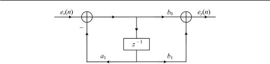
Figure 7.19 First-order IIR low-pass filters.
7.5.2 IIR filter algorithm of late reverberation
For the late diffused reverberation of a room, the temporal density of reflections from various directions increases as time is extended because of the increasing number of reflections from the boundary surfaces, as expressed in Equation (1.2.17). The overall energy of reverberations exponentially decays as time is prolonged because of the absorption of boundary surfaces. Late reverberation signals can be simulated with various perceived-based reverberation algorithms based on the statistical acoustic parameters of reverberation sound fields. Reverberation signals with a certain temporal density of reflections are enough to enhance auditory perceptions because of the limited resolution of human hearing. Schroeder (1962) suggested that a temporal density of not less than 1000/s is enough. On the basis of the results of psychoacoustic experiments, Kuttruff (2009) suggested a limit of 2000/s. Some other studies have also suggested a temporal density of ≥4000/s (Rubak and Johansen, 1998).
A plain reverberation algorithm simulates the successive reflections and decay in a room. It is implemented by combining the outputs of an infinite number of delay lines with lengths of m, 2m, 3m… samples and gains of g, g2, g3 …. (g < 1) relative to the original signal ex(n)
|
|
|
|
|
|
|
|
|
|
ey n ex n g |
q |
ex n qm . |
(7.5.21) |
||||||
|
|
||||||||
q 1 |
|
|
|
|
|
|
|
||
Equation (7.5.21) can be written in a recursive form; thus, |
|
||||||||
ey n ex n gey n m . |
(7.5.22) |
||||||||
Correspondingly, the impulse response and system function are |
|
||||||||
|
|
|
|
|
|
|
|
(7.5.23) |
|
|
|
|
|
|
q |
|
|
|
|
hREV n n g n qm , |
|
||||||||
q 1 |
|
|
|
|
|
|
|||
|
|
|
|
|
|
|
|
|
(7.5.24) |
HREV z 1 g |
q |
|
qm |
1 |
|
||||
|
z |
|
|
|
|
|
. |
|
|
|
|
|
|
1 gz m |
|
||||
q 1 |
|
|
|
|
|
|
|
|
|
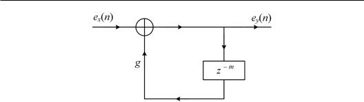
The impulse response hREV(n) in Equation (7.5.23) consists of an infinite series of unit impulses weighted with an infinite power series of g. The algorithm given by Equation (7.5.23) is called the plain reverberation algorithm, which is implemented by the IIR filter structure shown in Figure 7.20. The structure comprises a feedback loop with an m-sample

292 Spatial Sound
Figure 7.20 IIR filter structure for the plain reverberation algorithm.
delay line and g. The input and output of Figure 7.20 satisfy Equation (7.5.21), and this conclusion is easy to prove.
Equation (7.5.23) shows that each simulated reflection is delayed by m samples and attenuated g times compared with the preceding reflection. The magnitude of the qth reflection is gq times that of direct sound. As stated in Section 1.2.4, the reverberation time of the plain reverberation algorithm is evaluated by assuming 20 log10gq = −60 (dB):
T60 |
3m |
. |
(7.5.25) |
|
fs log10 g |
||||
|
|
|
For a given sampling frequency and delay line length m, T60 increases with the feedback g. The plain reverberation algorithm is simple with adjustable reverberation time and accommodates the exponential energy decay of natural reverberation. However, it suffers from the
following drawbacks:
1.Reverberation time is frequency independent, preventing it from simulating frequencydependent reverberation time caused by surface and air absorptions, which usually decrease as frequency increases in real rooms.
2.The equal time interval between two successive reflections tends to create fluttering.
Moreover, the simulated reflection density fs/m is usually small and invariable with time, which contradicts the phenomenon of increasing reflection density with time in real rooms.
3.The system function HREV(z) in Equation (7.5.24) includes m poles located at an equal interval in a circle with the radius g1/m in the Z-plane:
zp g |
1/m |
|
2 p |
p 0, 1, 2 m 1 . |
(7.5.26) |
|
|
exp j |
m |
|
|||
|
|
|
|
|
|
These poles cause the response magnitude |HREV(ω)| to vary with frequency, resulting in comb filtering characteristics similar to those shown in Figure 7.17(b). These characteristics cause subjective coloration in timbre. The peaks in |HREV(ω)| correspond to the poles of HREV(z). The digital angular frequencies of peaks are evaluated by substituting z = exp(jω) in Equation (7.5.26) as
p |
2 p |
p 0, 1 m 1 . |
(7.5.27) |
|
m |
|
|
A delay less than m = 44 in the plain reverberation algorithm is needed to obtain the temporal density of reflections larger than 1000/s at a sampling frequency of 44.1 kHz.

Microphone and signal simulation techniques 293
Accordingly, in Equation (7.5.25), g = 0.9966 is needed to simulate the reverberation time of T60 = 2 s. In this case, the poles in Equation (7.5.26) are located close to the unit circle | z | = 1 in the Z-plane and lead to instability in the IIR filter. For a given reverberation time T60, the delay m is increased, and g is reduced to improve the stability of the IIR filter. However, this process in turn reduces the temporal density of reflections. As such, using a single plain reverberation unit for late reflection simulation often causes perceivable artifacts. This problem prompts the improvement of the plain reverberation algorithm.
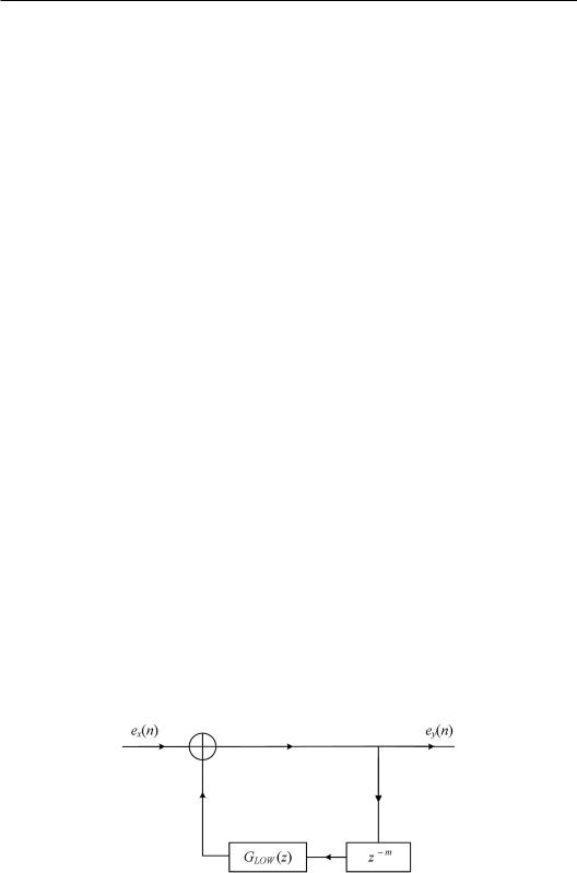
g in Equation (7.5.25) controls reverberation time. The low-pass reverberation algorithm shown in Figure 7.21 is implemented to simulate the surface and air absorption-induced decrease in reverberation time at high frequencies, where g in Figure 7.20 is replaced with a low-pass filter unit GLOW(z) (Moorer, 1979). The impulse response and system function of the low-pass reverberation algorithm are given by
hREV n
n gLOW n m gLOW n t gLOW n 2m gLOW n t gLOW n t gLOW n 3m .. ,
HREV z |
|
1 |
|
|
, |
1 |
GLOW |
z z |
m |
||
|
|
|
(7.5.28)
(7.5.29)
where gLOW(n) is the impulse response related to the low-pass filter GLOW(z), and “ t” denotes convolution. Similar to the case in Equation (7.5.19), the low-pass filter unit can be imple-
mented by an FIR or IIR structure and not repeated here.
In addition to the decrease in reverberation time at high frequencies, the reflection density in the low-pass reverberation algorithm increases with time. This behavior is consistent with the characteristics of late reflections in real rooms. High-order reflections in the low-pass reverberation algorithm are simulated through multiple convolutions with gLOW(n), which increases the temporal density of reflections.
To produce a flat static magnitude response and reduce the perceived timbre coloration, Schroeder (1962) proposed the well-known all-pass reverberation algorithm. The impulse response and system function of this algorithm are given by
|
|
g z m |
|
|
B2 |
|
|
|
|
||||
|
|
|
|
|
q |
|
qm |
||||||
HREV z |
|
|
|
|
B1 |
|
|
B1 B2 B2 g |
z |
|
|||
1 gz m |
|
1 gz m |
(7.5.30) |
||||||||||
|
|
|
|
|
|
|
|
1 g2 |
|
q 1 |
|
||
B1 |
|
1 |
|
B2 |
|
, |
|
|
|
||||
g |
|
g |
|
|
|
||||||||
|
|
|
|
|
|
|
|
|
|
|
Figure 7.21 Low-pass reverberation algorithm.

294 Spatial Sound
|
|
hREV n B1 B2 n B2 gq n qm . |
(7.5.31) |
q 1
hREV(n) comprises an infinite series of unit impulses with time-decaying gains. The magnitude of the (q + 1)th reflected impulse is g times that of the qth reflected impulse. The magnitude response of the system satisfies the following equation:
|HREV | 1. |
(7.5.32) |
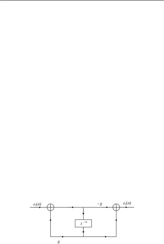
Therefore, the magnitude response is frequency independent. The all-pass reverberation algorithm can be implemented by the all-pass IIR filter structure shown in Figure 7.22. Equation (7.5.30) corresponds to the following input–output equation:
ey n gex n ex n m gey n m . |
(7.5.33) |
The all-pass reverberation algorithm cannot completely eliminate timbre coloration because of the short-term frequency analysis of human hearing. The flat static magnitude response of the algorithm is the consequence of long-term Fourier analysis.
Several all-pass reverberation units can be connected in series to increase reflection density. The ratios of delay in the all-pass reverberation unit are an irrational number so that reflections are inconsistent at the same instant. In practice, the Schroeder reverberation algorithm or the structure shown in Figure 7.23 is often adopted. The algorithm consists of several parallel plain reverberation units and a series connection of all-pass reverberation units. Reducing the coloration caused by comb filters necessitates using plain reverberation units with incommensurate delays, and the ratio between the largest and smallest delays is about 1.5. The temporal density of reflections caused by Q parallel plain reverberation units is given by
Q |
Q |
|
|||
dNdtR |
1 |
|
fs |
. |
(7.5.34) |
i |
mi |
||||
i 1 |
i 1 |
|
The density of the frequency model (eigenfrequenies) is given by
|
Q |
Q |
|
|
dNf |
i |
1 |
mi. |
(7.5.35) |
df |
fs |
|||
|
i 1 |
i 1 |
|
Figure 7.22 IIR filter structure of the all-pass reverberation algorithm.

Microphone and signal simulation techniques 295
Figure 7.23 Schroeder reverberation algorithm.
where τi = mi / fs is the delay of the ith plain reverberation unit, mi is the corresponding delay in the measured sample, and fs is the sampling frequency. The series connection of all-pass reverberation units is intended to increase the reflection density. Other elements in Figure 7.23 are similar to those in the aforementioned discussion. However, the simulated temporal density of reflections in Figure 7.23 is constant over time. The low-pass reverberation units in Figure 7.21 can be used to replace the plain reverberation units in Figure 7.23, thereby enabling the simulation of increasing reflection density with time in real rooms (Gardner, 2002). The parameters of the reverberation algorithm can be chosen in terms of statistical acoustic characteristics of a target hall. In practice, they can be chosen on the basis of various optimal perception methods (Bai and Bai, 2005).
On the basis of the work of Stanuter and Puckette (1982), Jot and Chaigne (1991) proposed a feedback delay network (FDN) structure of reverberation algorithms. As shown in Figure 7.24, the outputs of N parallel delay lines with different lengths are connected to all N inputs by an N × N feedback matrix [A]. The feedback matrix and delay in each delay line may be designed so that the outputs of delay lines are uncorrelated. Generally, the matrix [A] is chosen as a unitarity multiplying with a gain | g | < 1 to ensure the stability of the algorithm. The FDN structure is applicable to creating multichannel uncorrelated reverberations, and the inputs of N parallel delay lines can serve as multichannel signal inputs. Stanuter and Puckette illustrated an example of a four-input–four-output structure. Appropriate filters (such as low-pass filters) can be inserted before/after each delay line to simulate frequency-dependent reverberation time, but they also cause reflection density to increase with time. The FDN is the general form of an IIR reverberation structure. In the FDN structure with N inputs and N outputs, if the feedback matrix [A] is a diagonal matrix, channels are decoupled, and their structure is simplified into the case of N independent plain or low-pass reverberation units
Various reverberation algorithms in the time domain are discussed above. Some reverberation algorithms in the time-frequency domain have also been proposed to simulate the frequency-dependent decay of late reverberation in rooms. Nikolic (2002) used quadrature mirror filters (QMF) or wavelet decomposition to decompose the input signal into 2–16