
- •Preface
- •Introduction
- •1.1 Spatial coordinate systems
- •1.2 Sound fields and their physical characteristics
- •1.2.1 Free-field and sound waves generated by simple sound sources
- •1.2.2 Reflections from boundaries
- •1.2.3 Directivity of sound source radiation
- •1.2.4 Statistical analysis of acoustics in an enclosed space
- •1.2.5 Principle of sound receivers
- •1.3 Auditory system and perception
- •1.3.1 Auditory system and its functions
- •1.3.2 Hearing threshold and loudness
- •1.3.3 Masking
- •1.3.4 Critical band and auditory filter
- •1.4 Artificial head models and binaural signals
- •1.4.1 Artificial head models
- •1.4.2 Binaural signals and head-related transfer functions
- •1.5 Outline of spatial hearing
- •1.6 Localization cues for a single sound source
- •1.6.1 Interaural time difference
- •1.6.2 Interaural level difference
- •1.6.3 Cone of confusion and head movement
- •1.6.4 Spectral cues
- •1.6.5 Discussion on directional localization cues
- •1.6.6 Auditory distance perception
- •1.7 Summing localization and spatial hearing with multiple sources
- •1.7.1 Summing localization with two sound sources
- •1.7.2 The precedence effect
- •1.7.3 Spatial auditory perceptions with partially correlated and uncorrelated source signals
- •1.7.4 Auditory scene analysis and spatial hearing
- •1.7.5 Cocktail party effect
- •1.8 Room reflections and auditory spatial impression
- •1.8.1 Auditory spatial impression
- •1.8.2 Sound field-related measures and auditory spatial impression
- •1.8.3 Binaural-related measures and auditory spatial impression
- •1.9.1 Basic principle of spatial sound
- •1.9.2 Classification of spatial sound
- •1.9.3 Developments and applications of spatial sound
- •1.10 Summary
- •2.1 Basic principle of a two-channel stereophonic sound
- •2.1.1 Interchannel level difference and summing localization equation
- •2.1.2 Effect of frequency
- •2.1.3 Effect of interchannel phase difference
- •2.1.4 Virtual source created by interchannel time difference
- •2.1.5 Limitation of two-channel stereophonic sound
- •2.2.1 XY microphone pair
- •2.2.2 MS transformation and the MS microphone pair
- •2.2.3 Spaced microphone technique
- •2.2.4 Near-coincident microphone technique
- •2.2.5 Spot microphone and pan-pot technique
- •2.2.6 Discussion on microphone and signal simulation techniques for two-channel stereophonic sound
- •2.3 Upmixing and downmixing between two-channel stereophonic and mono signals
- •2.4 Two-channel stereophonic reproduction
- •2.4.1 Standard loudspeaker configuration of two-channel stereophonic sound
- •2.4.2 Influence of front-back deviation of the head
- •2.5 Summary
- •3.1 Physical and psychoacoustic principles of multichannel surround sound
- •3.2 Summing localization in multichannel horizontal surround sound
- •3.2.1 Summing localization equations for multiple horizontal loudspeakers
- •3.2.2 Analysis of the velocity and energy localization vectors of the superposed sound field
- •3.2.3 Discussion on horizontal summing localization equations
- •3.3 Multiple loudspeakers with partly correlated and low-correlated signals
- •3.4 Summary
- •4.1 Discrete quadraphone
- •4.1.1 Outline of the quadraphone
- •4.1.2 Discrete quadraphone with pair-wise amplitude panning
- •4.1.3 Discrete quadraphone with the first-order sound field signal mixing
- •4.1.4 Some discussions on discrete quadraphones
- •4.2 Other horizontal surround sounds with regular loudspeaker configurations
- •4.2.1 Six-channel reproduction with pair-wise amplitude panning
- •4.2.2 The first-order sound field signal mixing and reproduction with M ≥ 3 loudspeakers
- •4.3 Transformation of horizontal sound field signals and Ambisonics
- •4.3.1 Transformation of the first-order horizontal sound field signals
- •4.3.2 The first-order horizontal Ambisonics
- •4.3.3 The higher-order horizontal Ambisonics
- •4.3.4 Discussion and implementation of the horizontal Ambisonics
- •4.4 Summary
- •5.1 Outline of surround sounds with accompanying picture and general uses
- •5.2 5.1-Channel surround sound and its signal mixing analysis
- •5.2.1 Outline of 5.1-channel surround sound
- •5.2.2 Pair-wise amplitude panning for 5.1-channel surround sound
- •5.2.3 Global Ambisonic-like signal mixing for 5.1-channel sound
- •5.2.4 Optimization of three frontal loudspeaker signals and local Ambisonic-like signal mixing
- •5.2.5 Time panning for 5.1-channel surround sound
- •5.3 Other multichannel horizontal surround sounds
- •5.4 Low-frequency effect channel
- •5.5 Summary
- •6.1 Summing localization in multichannel spatial surround sound
- •6.1.1 Summing localization equations for spatial multiple loudspeaker configurations
- •6.1.2 Velocity and energy localization vector analysis for multichannel spatial surround sound
- •6.1.3 Discussion on spatial summing localization equations
- •6.1.4 Relationship with the horizontal summing localization equations
- •6.2 Signal mixing methods for a pair of vertical loudspeakers in the median and sagittal plane
- •6.3 Vector base amplitude panning
- •6.4 Spatial Ambisonic signal mixing and reproduction
- •6.4.1 Principle of spatial Ambisonics
- •6.4.2 Some examples of the first-order spatial Ambisonics
- •6.4.4 Recreating a top virtual source with a horizontal loudspeaker arrangement and Ambisonic signal mixing
- •6.5 Advanced multichannel spatial surround sounds and problems
- •6.5.1 Some advanced multichannel spatial surround sound techniques and systems
- •6.5.2 Object-based spatial sound
- •6.5.3 Some problems related to multichannel spatial surround sound
- •6.6 Summary
- •7.1 Basic considerations on the microphone and signal simulation techniques for multichannel sounds
- •7.2 Microphone techniques for 5.1-channel sound recording
- •7.2.1 Outline of microphone techniques for 5.1-channel sound recording
- •7.2.2 Main microphone techniques for 5.1-channel sound recording
- •7.2.3 Microphone techniques for the recording of three frontal channels
- •7.2.4 Microphone techniques for ambience recording and combination with frontal localization information recording
- •7.2.5 Stereophonic plus center channel recording
- •7.3 Microphone techniques for other multichannel sounds
- •7.3.1 Microphone techniques for other discrete multichannel sounds
- •7.3.2 Microphone techniques for Ambisonic recording
- •7.4 Simulation of localization signals for multichannel sounds
- •7.4.1 Methods of the simulation of directional localization signals
- •7.4.2 Simulation of virtual source distance and extension
- •7.4.3 Simulation of a moving virtual source
- •7.5 Simulation of reflections for stereophonic and multichannel sounds
- •7.5.1 Delay algorithms and discrete reflection simulation
- •7.5.2 IIR filter algorithm of late reverberation
- •7.5.3 FIR, hybrid FIR, and recursive filter algorithms of late reverberation
- •7.5.4 Algorithms of audio signal decorrelation
- •7.5.5 Simulation of room reflections based on physical measurement and calculation
- •7.6 Directional audio coding and multichannel sound signal synthesis
- •7.7 Summary
- •8.1 Matrix surround sound
- •8.1.1 Matrix quadraphone
- •8.1.2 Dolby Surround system
- •8.1.3 Dolby Pro-Logic decoding technique
- •8.1.4 Some developments on matrix surround sound and logic decoding techniques
- •8.2 Downmixing of multichannel sound signals
- •8.3 Upmixing of multichannel sound signals
- •8.3.1 Some considerations in upmixing
- •8.3.2 Simple upmixing methods for front-channel signals
- •8.3.3 Simple methods for Ambient component separation
- •8.3.4 Model and statistical characteristics of two-channel stereophonic signals
- •8.3.5 A scale-signal-based algorithm for upmixing
- •8.3.6 Upmixing algorithm based on principal component analysis
- •8.3.7 Algorithm based on the least mean square error for upmixing
- •8.3.8 Adaptive normalized algorithm based on the least mean square for upmixing
- •8.3.9 Some advanced upmixing algorithms
- •8.4 Summary
- •9.1 Each order approximation of ideal reproduction and Ambisonics
- •9.1.1 Each order approximation of ideal horizontal reproduction
- •9.1.2 Each order approximation of ideal three-dimensional reproduction
- •9.2 General formulation of multichannel sound field reconstruction
- •9.2.1 General formulation of multichannel sound field reconstruction in the spatial domain
- •9.2.2 Formulation of spatial-spectral domain analysis of circular secondary source array
- •9.2.3 Formulation of spatial-spectral domain analysis for a secondary source array on spherical surface
- •9.3 Spatial-spectral domain analysis and driving signals of Ambisonics
- •9.3.1 Reconstructed sound field of horizontal Ambisonics
- •9.3.2 Reconstructed sound field of spatial Ambisonics
- •9.3.3 Mixed-order Ambisonics
- •9.3.4 Near-field compensated higher-order Ambisonics
- •9.3.5 Ambisonic encoding of complex source information
- •9.3.6 Some special applications of spatial-spectral domain analysis of Ambisonics
- •9.4 Some problems related to Ambisonics
- •9.4.1 Secondary source array and stability of Ambisonics
- •9.4.2 Spatial transformation of Ambisonic sound field
- •9.5 Error analysis of Ambisonic-reconstructed sound field
- •9.5.1 Integral error of Ambisonic-reconstructed wavefront
- •9.5.2 Discrete secondary source array and spatial-spectral aliasing error in Ambisonics
- •9.6 Multichannel reconstructed sound field analysis in the spatial domain
- •9.6.1 Basic method for analysis in the spatial domain
- •9.6.2 Minimizing error in reconstructed sound field and summing localization equation
- •9.6.3 Multiple receiver position matching method and its relation to the mode-matching method
- •9.7 Listening room reflection compensation in multichannel sound reproduction
- •9.8 Microphone array for multichannel sound field signal recording
- •9.8.1 Circular microphone array for horizontal Ambisonic recording
- •9.8.2 Spherical microphone array for spatial Ambisonic recording
- •9.8.3 Discussion on microphone array recording
- •9.9 Summary
- •10.1 Basic principle and implementation of wave field synthesis
- •10.1.1 Kirchhoff–Helmholtz boundary integral and WFS
- •10.1.2 Simplification of the types of secondary sources
- •10.1.3 WFS in a horizontal plane with a linear array of secondary sources
- •10.1.4 Finite secondary source array and effect of spatial truncation
- •10.1.5 Discrete secondary source array and spatial aliasing
- •10.1.6 Some issues and related problems on WFS implementation
- •10.2 General theory of WFS
- •10.2.1 Green’s function of Helmholtz equation
- •10.2.2 General theory of three-dimensional WFS
- •10.2.3 General theory of two-dimensional WFS
- •10.2.4 Focused source in WFS
- •10.3 Analysis of WFS in the spatial-spectral domain
- •10.3.1 General formulation and analysis of WFS in the spatial-spectral domain
- •10.3.2 Analysis of the spatial aliasing in WFS
- •10.3.3 Spatial-spectral division method of WFS
- •10.4 Further discussion on sound field reconstruction
- •10.4.1 Comparison among various methods of sound field reconstruction
- •10.4.2 Further analysis of the relationship between acoustical holography and sound field reconstruction
- •10.4.3 Further analysis of the relationship between acoustical holography and Ambisonics
- •10.4.4 Comparison between WFS and Ambisonics
- •10.5 Equalization of WFS under nonideal conditions
- •10.6 Summary
- •11.1 Basic principles of binaural reproduction and virtual auditory display
- •11.1.1 Binaural recording and reproduction
- •11.1.2 Virtual auditory display
- •11.2 Acquisition of HRTFs
- •11.2.1 HRTF measurement
- •11.2.2 HRTF calculation
- •11.2.3 HRTF customization
- •11.3 Basic physical features of HRTFs
- •11.3.1 Time-domain features of far-field HRIRs
- •11.3.2 Frequency domain features of far-field HRTFs
- •11.3.3 Features of near-field HRTFs
- •11.4 HRTF-based filters for binaural synthesis
- •11.5 Spatial interpolation and decomposition of HRTFs
- •11.5.1 Directional interpolation of HRTFs
- •11.5.2 Spatial basis function decomposition and spatial sampling theorem of HRTFs
- •11.5.3 HRTF spatial interpolation and signal mixing for multichannel sound
- •11.5.4 Spectral shape basis function decomposition of HRTFs
- •11.6 Simplification of signal processing for binaural synthesis
- •11.6.1 Virtual loudspeaker-based algorithms
- •11.6.2 Basis function decomposition-based algorithms
- •11.7.1 Principle of headphone equalization
- •11.7.2 Some problems with binaural reproduction and VAD
- •11.8 Binaural reproduction through loudspeakers
- •11.8.1 Basic principle of binaural reproduction through loudspeakers
- •11.8.2 Virtual source distribution in two-front loudspeaker reproduction
- •11.8.3 Head movement and stability of virtual sources in Transaural reproduction
- •11.8.4 Timbre coloration and equalization in transaural reproduction
- •11.9 Virtual reproduction of stereophonic and multichannel surround sound
- •11.9.1 Binaural reproduction of stereophonic and multichannel sound through headphones
- •11.9.2 Stereophonic expansion and enhancement
- •11.9.3 Virtual reproduction of multichannel sound through loudspeakers
- •11.10.1 Binaural room modeling
- •11.10.2 Dynamic virtual auditory environments system
- •11.11 Summary
- •12.1 Physical analysis of binaural pressures in summing virtual source and auditory events
- •12.1.1 Evaluation of binaural pressures and localization cues
- •12.1.2 Method for summing localization analysis
- •12.1.3 Binaural pressure analysis of stereophonic and multichannel sound with amplitude panning
- •12.1.4 Analysis of summing localization with interchannel time difference
- •12.1.5 Analysis of summing localization at the off-central listening position
- •12.1.6 Analysis of interchannel correlation and spatial auditory sensations
- •12.2 Binaural auditory models and analysis of spatial sound reproduction
- •12.2.1 Analysis of lateral localization by using auditory models
- •12.2.2 Analysis of front-back and vertical localization by using a binaural auditory model
- •12.2.3 Binaural loudness models and analysis of the timbre of spatial sound reproduction
- •12.3 Binaural measurement system for assessing spatial sound reproduction
- •12.4 Summary
- •13.1 Analog audio storage and transmission
- •13.1.1 45°/45° Disk recording system
- •13.1.2 Analog magnetic tape audio recorder
- •13.1.3 Analog stereo broadcasting
- •13.2 Basic concepts of digital audio storage and transmission
- •13.3 Quantization noise and shaping
- •13.3.1 Signal-to-quantization noise ratio
- •13.3.2 Quantization noise shaping and 1-Bit DSD coding
- •13.4 Basic principle of digital audio compression and coding
- •13.4.1 Outline of digital audio compression and coding
- •13.4.2 Adaptive differential pulse-code modulation
- •13.4.3 Perceptual audio coding in the time-frequency domain
- •13.4.4 Vector quantization
- •13.4.5 Spatial audio coding
- •13.4.6 Spectral band replication
- •13.4.7 Entropy coding
- •13.4.8 Object-based audio coding
- •13.5 MPEG series of audio coding techniques and standards
- •13.5.1 MPEG-1 audio coding technique
- •13.5.2 MPEG-2 BC audio coding
- •13.5.3 MPEG-2 advanced audio coding
- •13.5.4 MPEG-4 audio coding
- •13.5.5 MPEG parametric coding of multichannel sound and unified speech and audio coding
- •13.5.6 MPEG-H 3D audio
- •13.6 Dolby series of coding techniques
- •13.6.1 Dolby digital coding technique
- •13.6.2 Some advanced Dolby coding techniques
- •13.7 DTS series of coding technique
- •13.8 MLP lossless coding technique
- •13.9 ATRAC technique
- •13.10 Audio video coding standard
- •13.11 Optical disks for audio storage
- •13.11.1 Structure, principle, and classification of optical disks
- •13.11.2 CD family and its audio formats
- •13.11.3 DVD family and its audio formats
- •13.11.4 SACD and its audio formats
- •13.11.5 BD and its audio formats
- •13.12 Digital radio and television broadcasting
- •13.12.1 Outline of digital radio and television broadcasting
- •13.12.2 Eureka-147 digital audio broadcasting
- •13.12.3 Digital radio mondiale
- •13.12.4 In-band on-channel digital audio broadcasting
- •13.12.5 Audio for digital television
- •13.13 Audio storage and transmission by personal computer
- •13.14 Summary
- •14.1 Outline of acoustic conditions and requirements for spatial sound intended for domestic reproduction
- •14.2 Acoustic consideration and design of listening rooms
- •14.3 Arrangement and characteristics of loudspeakers
- •14.3.1 Arrangement of the main loudspeakers in listening rooms
- •14.3.2 Characteristics of the main loudspeakers
- •14.3.3 Bass management and arrangement of subwoofers
- •14.4 Signal and listening level alignment
- •14.5 Standards and guidance for conditions of spatial sound reproduction
- •14.6 Headphones and binaural monitors of spatial sound reproduction
- •14.7 Acoustic conditions for cinema sound reproduction and monitoring
- •14.8 Summary
- •15.1 Outline of psychoacoustic and subjective assessment experiments
- •15.2 Contents and attributes for spatial sound assessment
- •15.3 Auditory comparison and discrimination experiment
- •15.3.1 Paradigms of auditory comparison and discrimination experiment
- •15.3.2 Examples of auditory comparison and discrimination experiment
- •15.4 Subjective assessment of small impairments in spatial sound systems
- •15.5 Subjective assessment of a spatial sound system with intermediate quality
- •15.6 Virtual source localization experiment
- •15.6.1 Basic methods for virtual source localization experiments
- •15.6.2 Preliminary analysis of the results of virtual source localization experiments
- •15.6.3 Some results of virtual source localization experiments
- •15.7 Summary
- •16.1.1 Application to commercial cinema and related problems
- •16.1.2 Applications to domestic reproduction and related problems
- •16.1.3 Applications to automobile audio
- •16.2.1 Applications to virtual reality
- •16.2.2 Applications to communication and information systems
- •16.2.3 Applications to multimedia
- •16.2.4 Applications to mobile and handheld devices
- •16.3 Applications to the scientific experiments of spatial hearing and psychoacoustics
- •16.4 Applications to sound field auralization
- •16.4.1 Auralization in room acoustics
- •16.4.2 Other applications of auralization technique
- •16.5 Applications to clinical medicine
- •16.6 Summary
- •References
- •Index

Microphone and signal simulation techniques 269
where θS is the target source azimuth in the original sound field. The normalized magnitude of C, L, and R microphone outputs maximize to a unit at θS = 0° and ±74°, respectively. When a target source is located midway between the main axis directions of two adjacent microphones, the normalized magnitudes of these two microphone outputs decrease by −3 dB with respect to the maximal on-axis output of a unit. A direct realization of the microphones with a second-order directivity may be difficult, but the signals given in Equation (7.2.1) can be derived for the outputs of an appropriate microphone array.
The virtual source localization performance in the reproduction of signals captured by the aforementioned coincident microphone array can be analyzed on the basis of the theorems presented in Section 3.2. Similar to the case of two-channel stereophonic sound, virtual source positions in the reproduction of three frontal channels may not be exactly consistent with those of the actual source at the original stage, but recreating the relative position distribution of virtual sources in reproduction is enough for live recording.
7.2.4 Microphone techniques for ambience recording and combination with frontal localization information recording
As stated in Section 7.2.3, two separate microphone arrays can be used to capture the frontal localization and ambient information in 5.1-channel recording. For live recording in a concert hall, ambiences are mainly reflections. In this case, ambient information is usually recorded with a wide-spaced microphone array arranged relatively far from the sources. The resultant decorrelated reflected signals recreate subjective sensations similar to those in the concert hall by using the direct method stated in Section 3.1. For 5.1-channel recording, the outputs of the ambient microphone array may be fed to the two surround channels only; accordingly, the three frontal channel microphones should be involved in the recording of ambient information. Alternatively, the outputs of ambient microphone array may be fed to frontal and surround channels to recreate the sensations of envelopment in reproduction. Many techniques for ambience recording have been developed, but some of them are based on experience rather than strict acoustic theory. The combinations of ambient microphone and frontal channel microphone arrays in Section 7.2.3 result in various practical 5.1-chan- nel microphone techniques. Furthermore, 5.1-channel recording with two separate microphone arrays is flexible. The performance of frontal localization information recording and ambience recording can be optimized separately with the less restrictive relation, and the direct-to-reverberation ratio in the recording is easily controlled. Various combinations of the frontal channel and ambient microphone arrays are available for a practical choice. An appropriate electronic delay may be supplemented to ambient signals to reduce their influence on frontal localization according to the precedence effect.
In the direct method of ambience recording, a pair of wide-spaced microphones is used to capture the decorrelated reflected signals. The theoretical basis of this method is expressed in Equations (1.2.29) and (1.2.30). An example of the combination of the frontal channel and ambient microphone arrays is the Fukada tree shown in Figure 7.9 (Fukada et al., 1997; Fukada, 2001). The configuration of three frontal microphones, including left (L), center (C), and right (R) microphones, is similar to that of the Decca tree. The Decca tree for twochannel stereophonic recording involves three omnidirectional microphones. The captured signals include frontal localization information and rear reflected information, and they are then reproduced by a pair of frontal stereophonic loudspeakers. In 5.1-channel reproduction, the frontal and rear information is reproduced by frontal and surround loudspeakers, respectively. Accordingly, three cardioid microphones with their main axes pointing to ± 55° to ± 65° in the LF and RF directions and to 0° in the C direction are used in the Fukada tree to capture the frontal source and frontal reflected signals. The directivity of the three frontal

270 Spatial Sound
Figure 7.9 Fukada tree.
microphones reduces the captured power of rear reflections. Two omnidirectional outrigger microphones, namely, LL and RR, are sometimes added outside the left and right microphones. The outputs of the outrigger microphones are usually panned between the left and left surround (or right and right surround) channels to increase the recording width of the frontal stage. A pair of left-back (surround) and right-back (surround) cardioid microphones, denoted by LS and RS, are used to record surround channels. They are located at the reverberation radius of the hall and spaced at a distance not less than the reverberation radius. Their main axes point to ±135° to ±150°. The outputs of LS and RS microphones are dominated by decorrelated reverberation from the rear. As stated in Section 7.2.3, the three frontal channel signals captured with wide-spaced microphone arrays such as Fukada tree result in the degraded quality of a virtual source. However, the three frontal microphones capture the ambience from the frontal at the same time. Wide-spaced microphone arrays reduce the cross-correlation among the outputs and then improve the auditory spatial impression in reproduction.
In addition to the wide-spaced microphone array, a near-coincident pair whose main axes pointing to the left-back and right-back directions or even a XY coincident pair (or its equivalent MS pair) can also be used to capture rear reflection. The combination of this near-coincident pair and three appropriate frontal channel microphones results in a complete 5.1-channel microphone technique. In contrast to the main microphone array in Section 7.2.2, the two back (surround) microphones in this technique are located far from the three frontal microphones (e.g., at a distance of 2–3 m or more). Accordingly, the outputs of two back microphones are mainly rear reflections, and they possess a low correlation with the three frontal channel outputs so that the summing localization between the frontal and rear channels is ignored. A pair of coincident or near-coincident rear microphones is not enough to record the decorrelated reverberation signals. However, when the outputs of these two microphones are fed to a pair of (rear) surround loudspeakers, a subjective sensation similar to those caused by reflections in a hall may be recreated by using the indirect method in Section 3.1. For example, the 5.1-channel recording technique suggested by DPA involves an array similar to the Decca tree to capture the frontal channel signals and a near-coincident ORTF pair to capture the surround channel signals (Nymand, 2003). The distance between the adjacent frontal microphones varies from 0.6 m to 1.2 m. The rear ORTF pair is located 8–10 m from the frontal array. Berg and Rumsey (2002) also used a near-coincident cardioid pair to capture rear reflections, but they utilized three coincident microphones for the recording of three frontal channels.

Microphone and signal simulation techniques 271
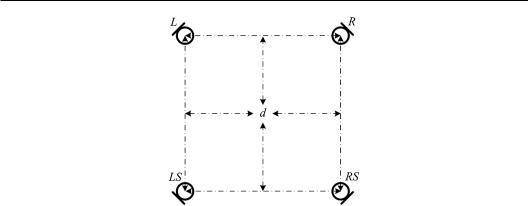
Figure 7.10 IRT cross.
Ambience can also be captured by four cardioid or omnidirectional microphones with a square arrangement. The four outputs are fed to the L, R, LS and the RS channels (Theile, 2001). The configuration of microphones is shown in Figure 7.10 and is called IRT-cross. When four cardioid microphones are used, the main axes of the microphones point to the LF, RF, LB and RB directions. The distance between the adjacent microphones varies from 0.25 m to 0.4 m. The distance of omnidirectional microphones is usually larger than that of cardioid microphones because the directivity of cardioid microphones also contributes to the decorrelation of the recorded signals in a reflected sound field. Theile combined the OCT frontal microphone array in Figure 7.7 with the IRT-cross in Figure 7.10 to construct a complete 5.1-channel microphone technique. The IRT-cross is located some distance behind the three frontal channel microphone array.
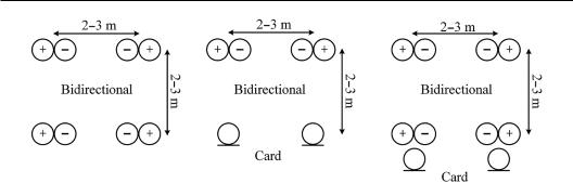
Hamasaki and Hiyama (2003) of NHK also proposed to use an array of four directional microphones with a square arrangement to capture the reflections in halls. This array is termed the Hamasaki square. The outputs of four microphones are fed to the L, R, and LS and the RS channels. Various configurations of the directivities of microphones are found in the Hamasaki square. Configuration 1 in Figure 7.11 (a) involves four bidirectional microphones with their main axes pointing to the lateral directions. It aims to capture lateral reflections and restrain the frontal direct sound and rear reflections to reduce their influence on frontal localization in reproduction. Configuration 2 in Figure 7.11 (b) involves two bidirectional microphones and two cardioid microphones. The main axes of cardioid microphones point to the rear directions. This configuration aims to capture rear reflections. Configuration 3 in Figure 7.11 (c) involves four bidirectional microphones with their main axes pointing to the lateral directions and two cardioid microphones with their main axes pointing to the rear. This configuration aims to capture lateral and rear reflections. The spaces between microphones in Figure 7.11 are chosen in terms of the correlation of the microphone outputs in the reverberation field, usually within the range of 2–3 m.
The Hamasaki square can be combined with other arrays to construct a complete 5.1-chan- nel microphone technique. Hamasaki’s original scheme was a combination of the frontal array in Figure 7.8 with a wide-spaced cardioid pair to capture rear/surround channel signals. The cardioid pair is located 2–3 m behind the frontal array and spaced apart at a distance of about 3 m. The main axes of the cardioid pair point to the left-back and right-back directions to capture the rear reflections. A Hamasaki square is shown in Figure 7.11(a) can be added to the above array to capture the ambient signals, and the outputs are mixed to the L, R, and the LS and the RS channels. The microphones in the Hamasaki square are spaced apart at a distance of 1 m (smaller than the latter choice of 2–3 m). In another scheme, Hamasaki also

272 Spatial Sound
Figure 7.11 The Hamasaki square: (a) configuration 1; (b) configuration 2; (c) configuration 3.
suggested using a five-microphone array similar to Figure 7.4 to capture the three frontal channel signals, but supercardioid microphones instead of cardioid microphones are used. The microphones are spaced apart at a distance of 1.5 m. An omnidirectional pair spaced apart by 4 m is also added. Their outputs are low-pass filtered with a crossover frequency of 250 Hz and mixed to the left and right channels to enhance the low-frequency recording. A Hamasaka square is placed 2–10 m behind the frontal array, which is determined on the basis of the required ratio of direct and reflected sounds in the captured signals.
Klepko (1997) proposed to use an omnidirectional pair placed in the two ears of an artificial head to capture ambient signals and combine them with a lined array of three microphones (Section 7.2.3) for 5.1-channel recording. The artificial head is placed 1.24 m behind the line array. As stated in Section 1.4, an artificial head simulates the anatomical structures of a real human from the perspective of acoustics. Binaural signals from artificial head recording are originally appropriate for headphone presentation. As stated in Section 11.8, a crosstalk cancellation processing should be supplemented when binaural signals are reproduced through loudspeakers. The effect of the head shadow partly plays a natural role in crosstalk cancellation because surround loudspeakers in 5.1-channel reproduction are arranged at the azimuths (±110°). Therefore, crosstalk cancellation processing is omitted in Klepko’s scheme. However, the final binaural signals in reproduction undergo the scattering and diffraction of the head/pinna twice (i.e., one is in the course of recording with the artificial head, and the other is in the course of reproduction to a listener, resulting in variation in the spectra in final binaural signals (pressures). Thus, timbre coloration occurs. Consequently, binaural signals from artificial head recording should be equalized.
The original purpose of artificial head recording is to make up for the deficiency of other methods, e.g., to recreate a virtual source within the rear region of ±90° with a pair of surround loudspeakers in 5.1-channel reproduction and to recreate the sensations similar to that in a hall by the indirect methods in Section 3.1. However, as stated in Section 11.8, even if crosstalk cancellation is included, the listening region of binaural signal reproduction via loudspeakers is narrowed. For a pair of surround loudspeakers with a wide span angle of 140°, a slight lateral translation of the head position spoils virtual source localization. On the other hand, the binaural signals captured by an artificial head in a nearly diffused reverberation field possess approximately equal power spectra and random phases. The scattering and diffracting effects of the artificial head enhance the randomness of binaural signals so that they are decorrelated. When reproduced by a pair of surround loudspeakers, these decorrelated signals lead to the sensation of envelopment in reproduction, and the perceived effect is less sensitive to the listening position. Therefore, using the artificial head for ambience recording is effective.