


Multichannel spatial surround sound 233
recreated by the two loudspeakers, and the signal for the other loudspeaker vanishes. If the target source is located between two adjacent loudspeakers in a horizontal plane, VBAP is simplified into horizontal pair-wise amplitude panning.
The resultant signal amplitudes A1, A2, and A3 should be normalized further. The normalized amplitudes of actual loudspeaker signals are A1, A2, and A3 multiplying Atotal. For constant-power normalization, the following equation is obtained:
Atotal |
1 |
, |
(6.3.5) |
A12 A22 A32 |
The aforementioned discussion is the basic principle of VBAP.
VBAP satisfies the low-frequency optimized criterion of the direction of the velocity localization vector. However, it does not satisfy the optimized criterion of the unit velocity vector magnitude rv = 1 except the target virtual source located in the loudspeaker direction. If the head rotates to an orientation so that ITDp vanishes, the lateral displacement of the perceived virtual source with respect to the fixed coordinate is identical to that of the target source. However, for a fixed head with a frontal orientation, the lateral displacement of the perceived virtual source may differ from that of the target source because of the mismatched ITDp in reproduction. Pulkki (2001a) also validated this result by using a binaural auditory model. In addition, the vertical displacement of the perceived virtual source may differ from that of the target source because of the mismatched variation in ITDp caused by head rotation. The accuracy of the perceived virtual source direction in reproduction depends on the positions of three active loudspeakers on a spherical surface and can be analyzed using the localization equations in Section 6.1.1. The situation here is similar to the cases of pair-wise amplitude panning in a horizontal plane (Section 4.1.2) or in a median plane (Section 6.2).
Four active loudspeakers with at least one out-of-phase loudspeaker signal are needed to further satisfy the optimized criterion of rv = 1. The function of an out-of-phase loudspeaker signal is similar to the cases of horizontal reproduction described in Sections 3.2.2 and 4.1.3. Out-of-phase loudspeaker signals are used in global or local Ambisonic signal mixing for horizontal and spatial reproduction, as discussed in Sections 4.3, 5.2.3, 5.2.4, and Section 6.4. The analysis here also reveals the difference between VBAP and Ambisonic signal mixing.
VBAP employs three active loudspeakers to recreate a virtual source within a spherical triangle formed by loudspeakers. Therefore, the error of the perceived virtual source direction is within the region bounded by active loudspeakers despite the position of a listener. The crosstalk from loudspeakers in opposite directions and a serious localization error in off-central listening position are averted. As the total number of loudspeakers increases, the active loudspeaker triangle grid becomes dense, and the localization error is further reduced. VBAP is simple and easily implemented in program production. Therefore, it possesses some advantages in practical uses. Some experiments on VBAP with various loudspeaker configurations have validated the aforementioned analysis (Pulkki, 2001a; Wendt et al., 2014).
6.4 SPATIAL AMBISONIC SIGNAL MIXING AND REPRODUCTION
6.4.1 Principle of spatial Ambisonics
Spatial Ambisonics is another typical multichannel spatial sound and signal mixing method (Gerzon, 1973). It was developed in the 1970s and originally termed Periphony. Currently, it is a hot topic in spatial sound. As an extension of horizontal Ambisonics, spatial Ambisonics involves the decomposition and reconstruction of a sound field by a series

234 Spatial Sound
of directional harmonics (spherical harmonic functions). Similar to horizontal Ambisonics, spatial Ambisonics can be analyzed with various mathematical and physical methods. A traditional analysis based on a virtual source localization theorem is addressed in this section, and a stricter analysis based on sound field reconstruction is presented in Chapter 9.
The first-order spatial Ambisonics involves four independent signals. If the maximal amplitude of independent signals is normalized to a unit, a set of normalized independent signals (amplitudes) can be chosen as
W 1 |
X cos S cos S |
Y sin S cos S |
Z sin S, |
(6.4.1) |
where (θS, ϕS) represent the azimuth and elevation of the target source in the original sound field. Equation (6.4.1) represents the signals captured by four coincident microphones in the original sound field. W is the signal from an omnidirectional microphone (spherical symmetrical directivity); X, Y, and Z are signals from three bidirectional microphones (symmetrical directivity around the polar axis) with their main axes pointing to the front, left, and top directions, respectively. The directional patterns of these four microphones are illustrated in Figure A.1 in Appendix A. W, X, Y, and Z also represent the pressure and the x (front-back), y (left-right), and z (up-down) components of the velocity of the medium in the original sound field, respectively.
In reproduction, M loudspeakers are arranged on a spherical surface around a listener. The distance from each loudspeaker to the origin (center of the sphere) satisfies the condition of a far-field distance. The direction of the ith loudspeaker is (θi,ϕi) with i = 0,1,2…M – 1, and loudspeaker signals can be written as a form of sound field signal mixing, i.e., as a linear combination of the independent signals W,X,Y, and Z given in Equation (6.4.1):
A |
, |
A |
D 1 |
|
, |
W D 1 |
|
, |
X D 2 |
|
, |
|
Y D 1 |
|
, |
Z |
|
|
|
|||||||||||||||||||||
i S |
S |
total |
|
00 |
|
i |
|
i |
|
|
|
11 |
i |
|
i |
|
|
|
11 |
|
i |
i |
|
|
|
10 |
i |
|
i |
|
|
|
|
|
||||||
|
|
|
D 1 |
|
, |
D 1 |
|
, |
|
cos |
|
cos |
D 2 |
|
, |
|
sin |
|
cos |
|
|
|
|
|||||||||||||||||
|
|
Atotal |
|
00 |
|
i |
|
i |
|
11 |
|
i |
i |
|
|
S |
|
|
S |
|
11 |
|
|
|
i |
i |
|
|
S |
|
|
S |
|
(6.4.2) |
||||||
|
|
|
|
|
|
1 |
|
, |
|
sin |
|
|
|
|
|
|
|
|
|
|
|
|
|
|
|
|
|
|
|
|
|
|
|
|
|
|
||||
|
|
|
|
D |
|
|
|
|
|
|
|
|
|
|
|
|
|
|
|
|
|
|
|
|
|
|
|
|
|
|
|
|
|
|||||||
|
|
|
|
10 |
|
i |
i |
|
S |
|
|
|
|
|
|
|
|
|
|
|
|
|
|
|
|
|
|
|
|
|
|
|
|
|
|
|||||
|
i 0, 1 |
|
|
|
|
|
|
|
|
|
|
|
|
|
|
|
|
|
|
|
|
|
|
|
|
|
|
|
|
|
|
|
|
|
|
|
||||
|
|
|
M 1 , |
|
|
|
|
|
|
|
|
|
|
|
|
|
|
|
|
|
|
|
|
|
|
|
|
|
|
|
|
|
|
|
||||||
where the decoding coefficients D 1 |
|
, |
, D 1 |
|
|
, |
|
, D 2 |
|
|
, |
|
, and D 1 |
|
, |
can |
||||||||||||||||||||||||
|
|
|
|
|
|
|
|
|
|
|
|
00 |
|
i |
|
i |
|
11 |
i |
i |
|
11 |
|
i |
|
i |
|
|
|
10 |
|
i |
i |
|
||||||
be chosen by using various methods depending on the loudspeaker configuration and optimized criteria for a reproduced sound field.
Generally, for left-right symmetrical loudspeaker configurations, decoding coefficients satisfy symmetrical relationships similar to those in Equations (5.2.16)–(5.2.18). If loudspeaker configurations are also up-down symmetric, for any pair of up-down symmetrical loudspeakers I and i′, their azimuths and elevations satisfy θi= θi′ and ϕi = −ϕi′, and
D 1 |
|
, |
D 1 |
|
i |
, |
|
||||
00 |
|
i |
i |
00 |
|
|
|
|
i |
|
|
D 1 |
|
, |
D 1 |
|
|
i |
, |
. |
|||
10 |
|
i |
i |
10 |
|
|
i |
|
|||
D 1 |
|
, |
D 1 |
|
, |
D 2 |
|
, |
D 2 |
|
, |
11 |
i |
i |
11 |
i |
i |
11 |
i |
i |
11 |
i |
i (6.4.3) |
Symmetry greatly simplifies the decoding coefficients.
The decoding coefficients in Equation (6.4.2) are solved in accordance with various optimized criteria. Similar to the case of horizontal Ambisonics with an irregular loudspeaker configuration in Section 5.2.3, the optimized criterion of the perceived virtual source direction

Multichannel spatial surround sound 235
matching that of a target source can be used when the head is fixed and when the head is turning at low frequencies; as such, θ I = θ′I = θS and ϕI = ϕ′I = ϕ″I = ϕS in Equations (6.1.11), (6.1.13), and (6.1.14). With these parameters, a set of linear equations for decoding coefficients can be obtained. Furthermore, θv= θS, ϕv = ϕS, and rv= 1 can be set in Equation (6.1.18) by using the optimized criterion of the velocity localization vector; the normalized pressure amplitude in the origin is set to a unit, so the following equation is obtained:
M 1 |
M 1 |
|
|
|
Ai S, S 1 |
Ai S, S cos i cos i cos S cos S |
|
|
|
i 0 |
i 0 |
. |
(6.4.4) |
|
M 1 |
M 1 |
|||
|
|
|||
Ai S, S sin i cos i sin S cos S |
Ai S, S sin i sin S |
|
|
|
i 0 |
i 0 |
|
|
Substituting Equation (6.4.2) into Equation (6.4.4) leads to a set of linear equations or a matrix equation for decoding coefficients:
3D |
total 3D |
3D |
3D |
|
(6.4.5) |
|
S |
A Y |
D |
S |
, |
||
|
where S′3D = [W, X, Y, Z]T is a 4 × 1 column matrix or vector composed of independent signals in Equation (6.4.1), the subscript “3D” denotes the case of three-dimensional spatial Ambisonics; and [D′3D] is an M ×4 decoding matrix to be solved:
|
D 1 |
|
, |
|
D 1 |
|
, |
|
D 2 |
|
, |
|
D 1 |
|
, |
|
|
|
||||
|
00 |
0 |
0 |
11 |
0 |
0 |
11 |
0 |
0 |
10 |
0 |
0 |
|
|
||||||||
|
D 1 |
, |
|
D 1 |
, |
|
D 2 |
, |
|
D 1 |
, |
|
|
. (6.4.6) |
||||||||
D3D |
|
00 |
1 |
1 |
|
11 |
1 |
1 |
11 |
1 |
1 |
|
10 |
1 |
1 |
|
||||||
|
|
|
|
|
|
|
|
|
|
|
|
|
|
|
|
|
|
|
|
|
|
|
D 1 |
|
|
, |
|
D 1 |
|
|
, |
|
D 2 |
|
|
, |
|
D 1 |
|
|
, |
|
|
|
|
|
00 |
|
M 1 |
M 1 |
11 |
|
M 1 |
M 1 |
11 |
|
M 1 |
M 1 |
10 |
|
M 1 |
M 1 |
|
|
||||
[Y′3D] is a 4 × M matrix with its entries related to the directions of loudspeakers:
|
|
1 |
1 |
|
1 |
|
|
|
|
|
cos 1 cos 1 |
|
cos M 1 cos M 1 |
|
|
Y3D |
cos 0 cos 0 |
|
|
||||
sin 0 cos 0 |
sin 1 cos 1 |
|
sin M 1 cos M 1 |
. |
(6.4.7) |
||
|
|
sin 0 |
sin 1 |
|
sin M 1 |
|
|
|
|
|
|
||||
Similar to the case of Equation (5.2.24), for M> 4, the decoding coefficients in Equation (6.4.5) can be solved from the following pseudo-inverse methods if the loudspeaker configuration is chosen appropriately so that the matrix [Y′3D] is well conditioned (Section 9.4.1):
T |
|
T |
|
1 |
|
Atotal D3D pinv Y3D Y3D |
Y3D Y3D . |
(6.4.8) |
|||
|
|
|
|
|
|
The solution given in Equation (6.4.8) satisfies the condition of constant-amplitude normalization. For M = 4, the decoding coefficients can be directly solved from the inverse of
236 Spatial Sound
the matrix [Y′3D]. Except for some regular loudspeaker configurations, the solution shown in Equation (6.4.8) usually does not satisfy the criterion of constant power in reproduction:
M 1 |
|
Pow Ai2 const. |
(6.4.9) |
i 0
For the solution expressed in Equation (6.4.8), the direction of the energy localization vector evaluated using Equation (6.1.20) generally does not coincide with that of the velocity localization vector, i.e., (θE, ϕE) ≠ (θv, ϕv). However, as indicated by Equation (6.4.4), the first-order spatial Ambisonics with a decoding matrix given by Equation (6.4.8) is an example in which Equations (6.1.11), (6.1.13), and (6.1.14) are consistent. In other words, the first-order spatial Ambisonics creates ITDp, and its dynamic variation with head rotation and tilting that match with those of the target source at very low frequencies.
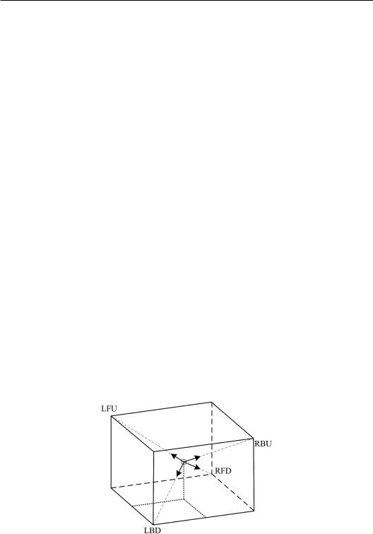
Similar to the case of horizontal Ambisonics (Section 4.3.1), spatial Ambisonics has various forms of independent signals. In principle, four independent linear combinations of W, X, Y, and Z can serve as a set of independent signals of spatial Ambisonics. Different sets of independent signals can be converted mutually. The decoding equations for different sets of independent signals are related via linear matrix transformation. In practice, four independent signals can be captured by four cardioid or subcardioid microphones with symmetrical directivity around the polar axis. The main axes of four microphones are pointed to the four non-parallel directions: left-front-up (LFU), left-back-down (LBD), right-front-down (RFD), and right-back-up (RBU) (Figure 6.7). The normalized amplitudes of microphone signals are
A |
|
A |
1 bcos |
|
|
i 0, 1, 2, 3. |
(6.4.10) |
i |
i |
mic |
i |
|
|
||
where 0.5 ≤ b ≤ 1, Ω′i′ is the angle between the target source direction and the main axis of the ith microphone, and Amic is a coefficient associated with the acoustic-electric efficiency or gain of microphones. The independent signals expressed in Equation (6.4.10) are termed A-format spatial Ambisonic signals.
Figure 6.7 Main axis directions of the four microphones for recording the A-format first-order spatial Ambisonic signals.
Multichannel spatial surround sound 237
W, X, Y, and Z given in Equation (6.4.1) can be conveniently chosen as the independent signals of the first-order spatial Ambisonics. W, X, Y, and Z can be derived from the signals presented in Equation (6.4.10) through linear transformation. Let
A |
A |
|
|
|
A |
A |
|
A |
A |
|
|
A |
A |
|
|
|
. (6.4.11) |
|||
LFU |
0 |
|
|
0 |
LBD |
1 |
1 |
RFD |
|
2 |
2 |
RBU |
3 |
3 |
|
|||||
The linear combinations of the four signals in Equation (6.4.1) yield |
|
|
|
|
||||||||||||||||
|
W |
|
|
|
|
|
|
|
4Amic |
|
|
|
|
|
|
|||||
|
|
ALFU ALBD ARFD ARBU |
|
|
|
|
|
|
||||||||||||
|
|
X |
|
|
|
|
|
|
|
|
4b |
Amic cos S cos S |
|
|
|
|
||||
|
|
|
3 |
|
|
|
|
|||||||||||||
|
|
|
ALFU ALBD ARFD ARBU |
|
|
|
|
|||||||||||||
|
|
Y |
|
|
|
|
|
|
|
|
4b |
Amic sin S cos S |
|
|
|
(6.4.12) |
||||
|
|
|
ALFU ALBD ARFD ARBU |
3 |
|
|
|
|
||||||||||||
|
|
|
|
|
|
|
|
|
|
|
|
4b |
Amic sin S. |
|
|
|
|
|
||
|
|
Z |
ALFU ALBD ARFD ARBU |
3 |
|
|
|
|
|
|||||||||||
The normalized independent signals W, X, Y, and Z are obtained by equalizing the signals in Equation (6.4.12) with an appropriate gain. In practice, the levels of X, Y, and Z are increased by 3 dB to ensure a diffused-field power response identical to that of the M signal. The independent signals are written as
W W 1 |
X 2X 2 cos S cos S |
Y 2Y 2 sin S cos S |
(6.4.13) |
|
|
2Z |
2 sin S . |
|
|
|
|
|||
Z |
|
|
||
The decoding equation should be appropriately changed to accommodate the independent signals in Equation (6.4.13). The spatial Ambisonic system with independent signals given by Equation (6.4.13) is termed the first-order B-format spatial Ambisonics (Gerzon, 1985).
The secondand higher-order directional harmonics (appendix A) are supplemented as new independent signals to improve the performance in reproduction, and the first-order spatial Ambisonics can be extended to the higher-order spatial Ambisonics. Under the optimized criterion of matching each order approximation of reproduced sound pressures with those of the target source within a given listening region and below a certain frequency limit, the decoding coefficients or matrix and loudspeaker signals are solved via a pseudoinverse method similar to Equation (6.4.8). This problem is addressed in Section 9.3.2. For the secondand higher-order spatial Ambisonics with decoding coefficients given in Equation (6.4.4), localization Equations (6.1.11), (6.1.13), and (6.1.14) yield consistent results. Equation (6.4.4) only specifies the zero and first-order decoding coefficients, flexibly leaving room for choosing the secondand higher-decoding coefficients.
Moreover, the equivalence between A-format and B-format spatial Ambisonics allows a post-equalization of recorded source signal at a given direction (Favrot and Faller, 2020). By using an appropriate matrix, the recorded B-format signals can be converted into a set of A-format signals with the main axis of polar pattern of one of A-format signal A′0( Ω′0) points to the concerned source direction. The resultant signal A′0( Ω′0) is equalized and, and the equalized signal along with the other un-equalized A-format signals are converted back into B-format signals by an invert matrix.