
- •Preface
- •Introduction
- •1.1 Spatial coordinate systems
- •1.2 Sound fields and their physical characteristics
- •1.2.1 Free-field and sound waves generated by simple sound sources
- •1.2.2 Reflections from boundaries
- •1.2.3 Directivity of sound source radiation
- •1.2.4 Statistical analysis of acoustics in an enclosed space
- •1.2.5 Principle of sound receivers
- •1.3 Auditory system and perception
- •1.3.1 Auditory system and its functions
- •1.3.2 Hearing threshold and loudness
- •1.3.3 Masking
- •1.3.4 Critical band and auditory filter
- •1.4 Artificial head models and binaural signals
- •1.4.1 Artificial head models
- •1.4.2 Binaural signals and head-related transfer functions
- •1.5 Outline of spatial hearing
- •1.6 Localization cues for a single sound source
- •1.6.1 Interaural time difference
- •1.6.2 Interaural level difference
- •1.6.3 Cone of confusion and head movement
- •1.6.4 Spectral cues
- •1.6.5 Discussion on directional localization cues
- •1.6.6 Auditory distance perception
- •1.7 Summing localization and spatial hearing with multiple sources
- •1.7.1 Summing localization with two sound sources
- •1.7.2 The precedence effect
- •1.7.3 Spatial auditory perceptions with partially correlated and uncorrelated source signals
- •1.7.4 Auditory scene analysis and spatial hearing
- •1.7.5 Cocktail party effect
- •1.8 Room reflections and auditory spatial impression
- •1.8.1 Auditory spatial impression
- •1.8.2 Sound field-related measures and auditory spatial impression
- •1.8.3 Binaural-related measures and auditory spatial impression
- •1.9.1 Basic principle of spatial sound
- •1.9.2 Classification of spatial sound
- •1.9.3 Developments and applications of spatial sound
- •1.10 Summary
- •2.1 Basic principle of a two-channel stereophonic sound
- •2.1.1 Interchannel level difference and summing localization equation
- •2.1.2 Effect of frequency
- •2.1.3 Effect of interchannel phase difference
- •2.1.4 Virtual source created by interchannel time difference
- •2.1.5 Limitation of two-channel stereophonic sound
- •2.2.1 XY microphone pair
- •2.2.2 MS transformation and the MS microphone pair
- •2.2.3 Spaced microphone technique
- •2.2.4 Near-coincident microphone technique
- •2.2.5 Spot microphone and pan-pot technique
- •2.2.6 Discussion on microphone and signal simulation techniques for two-channel stereophonic sound
- •2.3 Upmixing and downmixing between two-channel stereophonic and mono signals
- •2.4 Two-channel stereophonic reproduction
- •2.4.1 Standard loudspeaker configuration of two-channel stereophonic sound
- •2.4.2 Influence of front-back deviation of the head
- •2.5 Summary
- •3.1 Physical and psychoacoustic principles of multichannel surround sound
- •3.2 Summing localization in multichannel horizontal surround sound
- •3.2.1 Summing localization equations for multiple horizontal loudspeakers
- •3.2.2 Analysis of the velocity and energy localization vectors of the superposed sound field
- •3.2.3 Discussion on horizontal summing localization equations
- •3.3 Multiple loudspeakers with partly correlated and low-correlated signals
- •3.4 Summary
- •4.1 Discrete quadraphone
- •4.1.1 Outline of the quadraphone
- •4.1.2 Discrete quadraphone with pair-wise amplitude panning
- •4.1.3 Discrete quadraphone with the first-order sound field signal mixing
- •4.1.4 Some discussions on discrete quadraphones
- •4.2 Other horizontal surround sounds with regular loudspeaker configurations
- •4.2.1 Six-channel reproduction with pair-wise amplitude panning
- •4.2.2 The first-order sound field signal mixing and reproduction with M ≥ 3 loudspeakers
- •4.3 Transformation of horizontal sound field signals and Ambisonics
- •4.3.1 Transformation of the first-order horizontal sound field signals
- •4.3.2 The first-order horizontal Ambisonics
- •4.3.3 The higher-order horizontal Ambisonics
- •4.3.4 Discussion and implementation of the horizontal Ambisonics
- •4.4 Summary
- •5.1 Outline of surround sounds with accompanying picture and general uses
- •5.2 5.1-Channel surround sound and its signal mixing analysis
- •5.2.1 Outline of 5.1-channel surround sound
- •5.2.2 Pair-wise amplitude panning for 5.1-channel surround sound
- •5.2.3 Global Ambisonic-like signal mixing for 5.1-channel sound
- •5.2.4 Optimization of three frontal loudspeaker signals and local Ambisonic-like signal mixing
- •5.2.5 Time panning for 5.1-channel surround sound
- •5.3 Other multichannel horizontal surround sounds
- •5.4 Low-frequency effect channel
- •5.5 Summary
- •6.1 Summing localization in multichannel spatial surround sound
- •6.1.1 Summing localization equations for spatial multiple loudspeaker configurations
- •6.1.2 Velocity and energy localization vector analysis for multichannel spatial surround sound
- •6.1.3 Discussion on spatial summing localization equations
- •6.1.4 Relationship with the horizontal summing localization equations
- •6.2 Signal mixing methods for a pair of vertical loudspeakers in the median and sagittal plane
- •6.3 Vector base amplitude panning
- •6.4 Spatial Ambisonic signal mixing and reproduction
- •6.4.1 Principle of spatial Ambisonics
- •6.4.2 Some examples of the first-order spatial Ambisonics
- •6.4.4 Recreating a top virtual source with a horizontal loudspeaker arrangement and Ambisonic signal mixing
- •6.5 Advanced multichannel spatial surround sounds and problems
- •6.5.1 Some advanced multichannel spatial surround sound techniques and systems
- •6.5.2 Object-based spatial sound
- •6.5.3 Some problems related to multichannel spatial surround sound
- •6.6 Summary
- •7.1 Basic considerations on the microphone and signal simulation techniques for multichannel sounds
- •7.2 Microphone techniques for 5.1-channel sound recording
- •7.2.1 Outline of microphone techniques for 5.1-channel sound recording
- •7.2.2 Main microphone techniques for 5.1-channel sound recording
- •7.2.3 Microphone techniques for the recording of three frontal channels
- •7.2.4 Microphone techniques for ambience recording and combination with frontal localization information recording
- •7.2.5 Stereophonic plus center channel recording
- •7.3 Microphone techniques for other multichannel sounds
- •7.3.1 Microphone techniques for other discrete multichannel sounds
- •7.3.2 Microphone techniques for Ambisonic recording
- •7.4 Simulation of localization signals for multichannel sounds
- •7.4.1 Methods of the simulation of directional localization signals
- •7.4.2 Simulation of virtual source distance and extension
- •7.4.3 Simulation of a moving virtual source
- •7.5 Simulation of reflections for stereophonic and multichannel sounds
- •7.5.1 Delay algorithms and discrete reflection simulation
- •7.5.2 IIR filter algorithm of late reverberation
- •7.5.3 FIR, hybrid FIR, and recursive filter algorithms of late reverberation
- •7.5.4 Algorithms of audio signal decorrelation
- •7.5.5 Simulation of room reflections based on physical measurement and calculation
- •7.6 Directional audio coding and multichannel sound signal synthesis
- •7.7 Summary
- •8.1 Matrix surround sound
- •8.1.1 Matrix quadraphone
- •8.1.2 Dolby Surround system
- •8.1.3 Dolby Pro-Logic decoding technique
- •8.1.4 Some developments on matrix surround sound and logic decoding techniques
- •8.2 Downmixing of multichannel sound signals
- •8.3 Upmixing of multichannel sound signals
- •8.3.1 Some considerations in upmixing
- •8.3.2 Simple upmixing methods for front-channel signals
- •8.3.3 Simple methods for Ambient component separation
- •8.3.4 Model and statistical characteristics of two-channel stereophonic signals
- •8.3.5 A scale-signal-based algorithm for upmixing
- •8.3.6 Upmixing algorithm based on principal component analysis
- •8.3.7 Algorithm based on the least mean square error for upmixing
- •8.3.8 Adaptive normalized algorithm based on the least mean square for upmixing
- •8.3.9 Some advanced upmixing algorithms
- •8.4 Summary
- •9.1 Each order approximation of ideal reproduction and Ambisonics
- •9.1.1 Each order approximation of ideal horizontal reproduction
- •9.1.2 Each order approximation of ideal three-dimensional reproduction
- •9.2 General formulation of multichannel sound field reconstruction
- •9.2.1 General formulation of multichannel sound field reconstruction in the spatial domain
- •9.2.2 Formulation of spatial-spectral domain analysis of circular secondary source array
- •9.2.3 Formulation of spatial-spectral domain analysis for a secondary source array on spherical surface
- •9.3 Spatial-spectral domain analysis and driving signals of Ambisonics
- •9.3.1 Reconstructed sound field of horizontal Ambisonics
- •9.3.2 Reconstructed sound field of spatial Ambisonics
- •9.3.3 Mixed-order Ambisonics
- •9.3.4 Near-field compensated higher-order Ambisonics
- •9.3.5 Ambisonic encoding of complex source information
- •9.3.6 Some special applications of spatial-spectral domain analysis of Ambisonics
- •9.4 Some problems related to Ambisonics
- •9.4.1 Secondary source array and stability of Ambisonics
- •9.4.2 Spatial transformation of Ambisonic sound field
- •9.5 Error analysis of Ambisonic-reconstructed sound field
- •9.5.1 Integral error of Ambisonic-reconstructed wavefront
- •9.5.2 Discrete secondary source array and spatial-spectral aliasing error in Ambisonics
- •9.6 Multichannel reconstructed sound field analysis in the spatial domain
- •9.6.1 Basic method for analysis in the spatial domain
- •9.6.2 Minimizing error in reconstructed sound field and summing localization equation
- •9.6.3 Multiple receiver position matching method and its relation to the mode-matching method
- •9.7 Listening room reflection compensation in multichannel sound reproduction
- •9.8 Microphone array for multichannel sound field signal recording
- •9.8.1 Circular microphone array for horizontal Ambisonic recording
- •9.8.2 Spherical microphone array for spatial Ambisonic recording
- •9.8.3 Discussion on microphone array recording
- •9.9 Summary
- •10.1 Basic principle and implementation of wave field synthesis
- •10.1.1 Kirchhoff–Helmholtz boundary integral and WFS
- •10.1.2 Simplification of the types of secondary sources
- •10.1.3 WFS in a horizontal plane with a linear array of secondary sources
- •10.1.4 Finite secondary source array and effect of spatial truncation
- •10.1.5 Discrete secondary source array and spatial aliasing
- •10.1.6 Some issues and related problems on WFS implementation
- •10.2 General theory of WFS
- •10.2.1 Green’s function of Helmholtz equation
- •10.2.2 General theory of three-dimensional WFS
- •10.2.3 General theory of two-dimensional WFS
- •10.2.4 Focused source in WFS
- •10.3 Analysis of WFS in the spatial-spectral domain
- •10.3.1 General formulation and analysis of WFS in the spatial-spectral domain
- •10.3.2 Analysis of the spatial aliasing in WFS
- •10.3.3 Spatial-spectral division method of WFS
- •10.4 Further discussion on sound field reconstruction
- •10.4.1 Comparison among various methods of sound field reconstruction
- •10.4.2 Further analysis of the relationship between acoustical holography and sound field reconstruction
- •10.4.3 Further analysis of the relationship between acoustical holography and Ambisonics
- •10.4.4 Comparison between WFS and Ambisonics
- •10.5 Equalization of WFS under nonideal conditions
- •10.6 Summary
- •11.1 Basic principles of binaural reproduction and virtual auditory display
- •11.1.1 Binaural recording and reproduction
- •11.1.2 Virtual auditory display
- •11.2 Acquisition of HRTFs
- •11.2.1 HRTF measurement
- •11.2.2 HRTF calculation
- •11.2.3 HRTF customization
- •11.3 Basic physical features of HRTFs
- •11.3.1 Time-domain features of far-field HRIRs
- •11.3.2 Frequency domain features of far-field HRTFs
- •11.3.3 Features of near-field HRTFs
- •11.4 HRTF-based filters for binaural synthesis
- •11.5 Spatial interpolation and decomposition of HRTFs
- •11.5.1 Directional interpolation of HRTFs
- •11.5.2 Spatial basis function decomposition and spatial sampling theorem of HRTFs
- •11.5.3 HRTF spatial interpolation and signal mixing for multichannel sound
- •11.5.4 Spectral shape basis function decomposition of HRTFs
- •11.6 Simplification of signal processing for binaural synthesis
- •11.6.1 Virtual loudspeaker-based algorithms
- •11.6.2 Basis function decomposition-based algorithms
- •11.7.1 Principle of headphone equalization
- •11.7.2 Some problems with binaural reproduction and VAD
- •11.8 Binaural reproduction through loudspeakers
- •11.8.1 Basic principle of binaural reproduction through loudspeakers
- •11.8.2 Virtual source distribution in two-front loudspeaker reproduction
- •11.8.3 Head movement and stability of virtual sources in Transaural reproduction
- •11.8.4 Timbre coloration and equalization in transaural reproduction
- •11.9 Virtual reproduction of stereophonic and multichannel surround sound
- •11.9.1 Binaural reproduction of stereophonic and multichannel sound through headphones
- •11.9.2 Stereophonic expansion and enhancement
- •11.9.3 Virtual reproduction of multichannel sound through loudspeakers
- •11.10.1 Binaural room modeling
- •11.10.2 Dynamic virtual auditory environments system
- •11.11 Summary
- •12.1 Physical analysis of binaural pressures in summing virtual source and auditory events
- •12.1.1 Evaluation of binaural pressures and localization cues
- •12.1.2 Method for summing localization analysis
- •12.1.3 Binaural pressure analysis of stereophonic and multichannel sound with amplitude panning
- •12.1.4 Analysis of summing localization with interchannel time difference
- •12.1.5 Analysis of summing localization at the off-central listening position
- •12.1.6 Analysis of interchannel correlation and spatial auditory sensations
- •12.2 Binaural auditory models and analysis of spatial sound reproduction
- •12.2.1 Analysis of lateral localization by using auditory models
- •12.2.2 Analysis of front-back and vertical localization by using a binaural auditory model
- •12.2.3 Binaural loudness models and analysis of the timbre of spatial sound reproduction
- •12.3 Binaural measurement system for assessing spatial sound reproduction
- •12.4 Summary
- •13.1 Analog audio storage and transmission
- •13.1.1 45°/45° Disk recording system
- •13.1.2 Analog magnetic tape audio recorder
- •13.1.3 Analog stereo broadcasting
- •13.2 Basic concepts of digital audio storage and transmission
- •13.3 Quantization noise and shaping
- •13.3.1 Signal-to-quantization noise ratio
- •13.3.2 Quantization noise shaping and 1-Bit DSD coding
- •13.4 Basic principle of digital audio compression and coding
- •13.4.1 Outline of digital audio compression and coding
- •13.4.2 Adaptive differential pulse-code modulation
- •13.4.3 Perceptual audio coding in the time-frequency domain
- •13.4.4 Vector quantization
- •13.4.5 Spatial audio coding
- •13.4.6 Spectral band replication
- •13.4.7 Entropy coding
- •13.4.8 Object-based audio coding
- •13.5 MPEG series of audio coding techniques and standards
- •13.5.1 MPEG-1 audio coding technique
- •13.5.2 MPEG-2 BC audio coding
- •13.5.3 MPEG-2 advanced audio coding
- •13.5.4 MPEG-4 audio coding
- •13.5.5 MPEG parametric coding of multichannel sound and unified speech and audio coding
- •13.5.6 MPEG-H 3D audio
- •13.6 Dolby series of coding techniques
- •13.6.1 Dolby digital coding technique
- •13.6.2 Some advanced Dolby coding techniques
- •13.7 DTS series of coding technique
- •13.8 MLP lossless coding technique
- •13.9 ATRAC technique
- •13.10 Audio video coding standard
- •13.11 Optical disks for audio storage
- •13.11.1 Structure, principle, and classification of optical disks
- •13.11.2 CD family and its audio formats
- •13.11.3 DVD family and its audio formats
- •13.11.4 SACD and its audio formats
- •13.11.5 BD and its audio formats
- •13.12 Digital radio and television broadcasting
- •13.12.1 Outline of digital radio and television broadcasting
- •13.12.2 Eureka-147 digital audio broadcasting
- •13.12.3 Digital radio mondiale
- •13.12.4 In-band on-channel digital audio broadcasting
- •13.12.5 Audio for digital television
- •13.13 Audio storage and transmission by personal computer
- •13.14 Summary
- •14.1 Outline of acoustic conditions and requirements for spatial sound intended for domestic reproduction
- •14.2 Acoustic consideration and design of listening rooms
- •14.3 Arrangement and characteristics of loudspeakers
- •14.3.1 Arrangement of the main loudspeakers in listening rooms
- •14.3.2 Characteristics of the main loudspeakers
- •14.3.3 Bass management and arrangement of subwoofers
- •14.4 Signal and listening level alignment
- •14.5 Standards and guidance for conditions of spatial sound reproduction
- •14.6 Headphones and binaural monitors of spatial sound reproduction
- •14.7 Acoustic conditions for cinema sound reproduction and monitoring
- •14.8 Summary
- •15.1 Outline of psychoacoustic and subjective assessment experiments
- •15.2 Contents and attributes for spatial sound assessment
- •15.3 Auditory comparison and discrimination experiment
- •15.3.1 Paradigms of auditory comparison and discrimination experiment
- •15.3.2 Examples of auditory comparison and discrimination experiment
- •15.4 Subjective assessment of small impairments in spatial sound systems
- •15.5 Subjective assessment of a spatial sound system with intermediate quality
- •15.6 Virtual source localization experiment
- •15.6.1 Basic methods for virtual source localization experiments
- •15.6.2 Preliminary analysis of the results of virtual source localization experiments
- •15.6.3 Some results of virtual source localization experiments
- •15.7 Summary
- •16.1.1 Application to commercial cinema and related problems
- •16.1.2 Applications to domestic reproduction and related problems
- •16.1.3 Applications to automobile audio
- •16.2.1 Applications to virtual reality
- •16.2.2 Applications to communication and information systems
- •16.2.3 Applications to multimedia
- •16.2.4 Applications to mobile and handheld devices
- •16.3 Applications to the scientific experiments of spatial hearing and psychoacoustics
- •16.4 Applications to sound field auralization
- •16.4.1 Auralization in room acoustics
- •16.4.2 Other applications of auralization technique
- •16.5 Applications to clinical medicine
- •16.6 Summary
- •References
- •Index

Multichannel spatial surround sound 225
axis, the dynamic ITDp variation provides information that the virtual source deviates from the direct front to a high or low elevation in the median plane. This deviation increases as the half-span angle θ0 of the loudspeaker pair increases. For a pair of horizontal loudspeakers arranged at the two sides with ±θ0 = ±90°, Equation (6.1.28) yields cosϕ′I = 0, and the perceived virtual source is located at the top (or bottom) direction.
3. The result of Equation (6.1.29) is inconsistent with that of Equation (6.1.28), indicating that the head tilting around the front-back axis fails to provide consistent information for up-down discrimination.
The virtual source-elevated effect also occurs in the case of regular horizontal loudspeaker configurations with more loudspeakers (such as four) and identical signal amplitudes. In this case, ITDp and its dynamic variation with head rotation on a vertical axis vanish, and this observation only matches with a real source in the top or bottom direction. However, Equation (6.1.24) provides an inconsistent or conflicting information on sin I 0 and fails to yield consistent information on up-down discrimination. This inconsistency reveals the limitation of the analysis in this section. On the other hand, the virtual source-elevated effect is applicable to recreate the perception of “flying over” with a horizontal loudspeaker configuration (Jot et al., 1999). A similar method is also applicable to an irregular loudspeaker configuration in a horizontal plane.
The above example indicates that the experimental results of a virtual source elevated in a horizontal loudspeaker arrangement can be partly and qualitatively interpreted by the dynamic cue caused by head turning. Some quantitative differences may be observed between the theoretical and experimental results, but the above analysis is at least qualitatively consistent with Wallach’s hypothesis, that is, the head rotation around the vertical axis provides information on the vertical displacement of a sound source from the horizontal plane. The virtual source elevated in a horizontal loudspeaker arrangement may be a comprehensive consequence of multiple cues, especially for wideband stimuli. For example, the scattering and diffraction of the torso do not provide information that the virtual source is located below the horizontal plane. The auditory system has adapted to a natural environment with sound sources on the top rather than below directions. However, the effect of multiple localization cues may cause a quantitative difference between the practical perceived directions and those predicted by Equations (6.1.27), (6.1.28), and (6.1.29). Moreover, other studies have interpreted the virtual source-elevated effect with a spectral cue or an interchannel crosstalk (Lee, 2017). Therefore, the analysis in this section is partly based on some hypotheses and thus incomplete; more psychoacoustic validations and corrections are required.
6.2 SIGNAL MIXING METHODS FOR A PAIR OF VERTICAL LOUDSPEAKERS IN THE MEDIAN AND SAGITTAL PLANE
The summing localization and other spatial auditory perceptions with a pair of loudspeakers in the horizontal plane are analyzed in Section 1.7.1 and in Chapters 2 to 5. They include recreating a virtual source between loudspeakers with pair-wise amplitude and time panning and recreating spatial auditory perceptions with decorrelated loudspeaker signals. These methods are applicable to two-channel stereophonic and horizontal surround sound reproduction. In multichannel spatial surround sound, a virtual source should also be recreated in the median plane and other sagittal planes with a pair of adjacent loudspeakers in different elevations. The feasibility of this method is analyzed in the following section. A comparison between the analysis and experiment also validates or reveals the limitations of the localization theorem in Section 6.1.

226 Spatial Sound
The virtual source localization equations in Section 6.1.1 are used to analyze the summing localization in the median plane at low frequencies (Rao and Xie, 2005; Xie and Rao, 2015; Xie et al., 2019). If all loudspeakers are arranged in the median plane with θi = 0° or 180°, then sinθi = 0 and i = 0,1…(M – 1). Equation (6.1.9) or (6.1.11) yields the interaural phase delay difference ITDp,SUM = 0, and the summing virtual source (if it exists) is located in the median plane with its perceived azimuth satisfying θI = 0° or 180°. Substituting this result into Equation (6.1.13) and letting θI = θ′I yield
M 1
Ai cos i cos i
cos I i 0 M 1 . (6.2.1)
Ai
i 0
When the virtual source is located in the frontal-median plane with θI = 0° or when the variation rate of ITDp,SUM with head rotation calculated from Equation (6.1.12) is negative, the positive sign should be chosen in Equation (6.2.1). Otherwise, the negative sign should be selected in Equation (6.2.1). According to Wallach’s hypothesis, Equation (6.2.1)is used to evaluate the elevation angle of the summing virtual source in the median plane quantitatively, and Equation (6.1.14) is applied to resolve the up-down ambiguity.
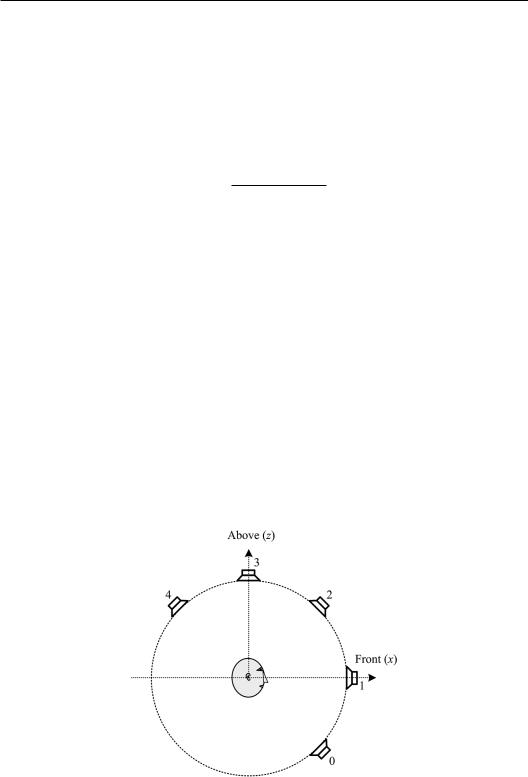
Equation (6.2.1) is used to analyze the examples of summing localization with two loudspeakers in the median plane. As shown in Figure 6.2, five loudspeakers numbered 0, 1, 2, 3, and 4 are arranged in the median plane. Loudspeakers 0, 1, and 2 are arranged in the frontalmedian plane with an azimuth of θi = 0° and elevations of ϕ0 = −ϕ2, ϕ1 = 0°, and 0° < ϕ2 < 90°, respectively. Loudspeaker 3 is arranged on the top with an azimuth of θ3= 0° and an elevation of ϕ3 = 90°. Loudspeaker 4 is arranged in the rear-median plane with an azimuth of θ4 = 180°and an elevation of ϕ4 = ϕ2. The normalized amplitudes of loudspeaker signals are denoted by A0, A1, A2, A3, and A4. For pair-wise amplitude panning between loudspeakers 1 and 2, A0, A3, and A4 vanish. In this case, Equation (6.1.14) yields sinϕ″I ≥ 0, and the virtual source is located in the upper half of the median plane. The variation rate of ITDp,SUM with
Figure 6.2 Five loudspeakers arranged in the median plane.

Multichannel spatial surround sound 227
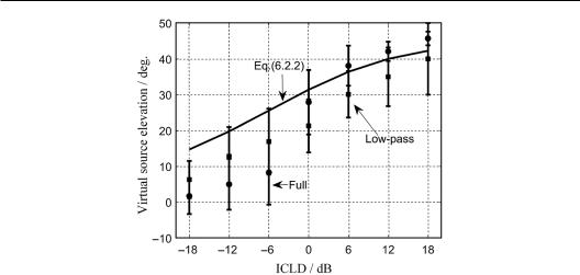
Figure 6.3 Elevation of a virtual source from the calculation and experiment for pair-wise amplitude panning between loudspeakers 1 and 2.
the head rotation calculated from Equation (6.1.12) is negative. Accordingly, the elevation of the virtual source in the frontal-median plane is evaluated from Equation (6.2.1) as
cos I |
A1 A2 cos 2 |
|
1 A2 /A1 cos 2 |
. |
(6.2.2) |
A1 A2 |
|
||||
|
|
1 A2 /A1 |
|
According to Equation (6.2.2), when the interchannel level difference (ICLD) d21 = 20log10(A2/A1) changes from −∞ dB to +∞ dB, the elevation of the virtual source varies from 0° to ϕ2. In this case, the panning can recreate a virtual source between the two adjacent loudspeakers. Figure 6.3 illustrates the result calculated from Equation (6.2.2) with ϕ2 = 45°.
Similar analyses indicate that pair-wise amplitude panning is also able to recreate a virtual source between two adjacent loudspeakers 0 and 1 or 2 and 3. By contrast, for pair-wise amplitude panning between loudspeakers 0 and 2, Equation (6.2.1) yields
cos I cos 2 cos 0. |
(6.2.3) |
Therefore, for a pair of up–down symmetrical loudspeakers, the virtual source is located in the direction of either loudspeaker 0 or 2 in spite of the interchannel level difference d20 = 20 log10(A2/A0), i.e., pair-wise amplitude panning fails to recreate a virtual source between two loudspeakers. This result is similar to the case when a pair of lateral loudspeakers with a front-back symmetrical arrangement fails to recreate a stable lateral virtual source (Section 4.1.2).
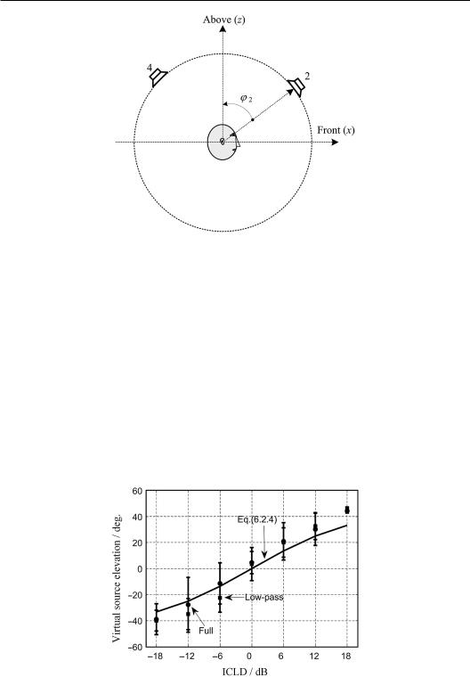
To analyze the pair-wise amplitude panning between loudspeakers 2 and 4, which have a front-back symmetrical arrangement, selecting a new elevation angle of −180° < φ ≤180° in the median plane is convenient. As shown in Figure 6.4, the new elevation angle is related to the default angle when θ = 0° and φ = 90° −ϕ and when θ = 180° and φ = −90° + ϕ. Therefore, the top, front, and back directions are denoted by φ = 0°, 90°, and −90°, respectively. As shown in Figure 6.4, the span angle between two loudspeakers is 2φ2 = 2(90°−ϕ2), where the elevation angles of the front and back loudspeakers are φ2 and φ4 = −φ2, respectively. For the normalized loudspeaker signal amplitudes A2 and A4, Equation (6.2.1) yields

228 Spatial Sound
Figure 6.4 Pair of loudspeakers with a front-back symmetrical arrangement in the median plane.
sin I |
A2 |
A4 |
sin 2 |
A2 /A4 |
1 |
sin 2. |
(6.2.4) |
A2 A4 |
|
|
|||||
|
|
A2 /A4 1 |
|
The form of Equation (6.2.4) is similar to the law of sine for stereophonic reproduction in the front horizontal plane described in Equation (2.1.6), resulting in a similar variation pattern of a virtual source angle with an interchannel level difference. Therefore, pair-wise amplitude panning can recreate a virtual source between a pair of loudspeakers with a frontback symmetrical arrangement in the median plane. For a half-span angle of φ2 = 45° between two loudspeakers, Figure 6.5 illustrates the variation in the perceived elevation angle φ′I with
ICLD = d24= 20 log10(A2 / A4) (dB). For d24 → + ∞, d24 = 0 and d24 → −∞, φ′I are 45°, 0°, and −45°, respectively.
The physical origins of Equation (6.2.4) are different from those of law of sine for stereophonic reproduction. The law of sine for stereophonic reproduction is derived from ITDp,
Figure 6.5 Elevation of a virtual source from the calculation and experiment for pair-wise amplitude panning between a pair of front-back symmetrical loudspeakers 2 and 4. In the figure, solid circle and square represent the results of full-bandwidth and low-pass filtered pink noise, respectively.

Multichannel spatial surround sound 229
which is a dominant cue for azimuthal localization at low frequencies. Equation (6.2.4) is derived from the variation in ITDp caused by head rotation, which is supposed to be a cue of elevation localization at low frequencies.
Figures 6.3 and 6.5 also illustrate the results of virtual source localization experiments, including the means and standard deviations from eight subjects. Pink noise with a fullaudible bandwidth and a 500 Hz low-pass filtered bandwidth are used as stimuli. The experimental results exhibit a tendency similar to that of the analysis. However, in Figure 6.3, for pink noise with a full-audible bandwidth and ICLD d21 = −6 dB, the elevation angle from the experimental result is closer to the direction of the front loudspeaker 1 than that from the analysis. This inconsistency may be attributed to the following reasons:
1. The accuracy of elevation localization is limited compared with that of azimuthal localization.
2. The approximate (shadowless) head model is used in the analysis.
3. The spectral cue in amplitude panning deviates from that of the target (real) source. The mismatched spectral cue may influence the localizations.
4. The localization information provided by head rotation is inconsistent with that given by tilting for pair-wise amplitude panning.
These reasons should be further examined experimentally.
For a pair of loudspeakers 0 and 2 with an up-down symmetrical arrangement in the median plane, the virtual source jumps from the direction of one loudspeaker to another when the ICLD changes. This experimental result is also consistent with that of theoretical analysis. In addition, the standard deviation of the experimental results in Figures 6.3 and 6.5 is larger than those of usual localization experiments in the horizontal plane. These standard deviations are larger probably because pair-wise amplitude panning with two loudspeakers in the median plane only provides information on dynamic ITDp variation for vertical localization. The perceived virtual source becomes blurry (for stimuli with a full-audible bandwidth) because of incorrect spectral information at high frequencies.
Some studies have explored the feasibility of recreating a virtual source between two loudspeakers in the median plane to develop spatial surround sound. The results vary across works. Pulkki (2001a) experimentally demonstrated that pair-wise amplitude panning fails to recreate virtual sources between two loudspeakers at ϕ = –15° and 30° in the median plane for pink-noise or narrow-band stimuli. This finding is similar to the case of pair-wise amplitude panning between loudspeakers 0 and 2 shown in Figure 6.2, although the loudspeaker configuration in Pulkki’s experiment was not completely symmetrical in the up-and-down direction. An analysis similar to that in Equation (6.2.3) can interpret Pulkki’s experimental results.
Wendt et al. (2014) conducted a virtual source localization experiment with a pair of loudspeakers at an elevation of ϕ = ±20° in the median plane. They used pink noise as a stimulus and set ICLD to 0, ±3, and ±6 dB. During the experiment, they instructed their subjects to keep their head immobile to the frontal orientation. The results indicated that the perceived elevation of a virtual source can be controlled by ICLD, but the quantitative results are obviously subject-dependent. Therefore, reproduction fails to create consistent localization cues.
In the development of advanced multichannel spatial sound, a series of virtual source localization experiments is also conducted to investigate the summing localization in the median plane (ITU-R Report, BS 2159-7, 2015). The experimental results from the ITU-R Report indicate that pair-wise amplitude panning for white noise stimuli can recreate a virtual source between two loudspeakers at ϕ = 0° and 30° or 0° and −30° in the median plane; however, it

230 Spatial Sound
fails to recreate a virtual source between two loudspeakers at ϕ = −30° and 30°. The results of the aforementioned analysis are also consistent with those in the ITU-R Report.
Lee (2014) investigated the perceived virtual source movement caused by ICLD in the median plane. They arranged two loudspeakers at elevations of 0° and 30° in the frontalmedian plane and used the signals of a cello and a bongo as stimuli. The results indicated that an ICLD of 6–7 dB is enough to make the virtual source fully move in the direction of either loudspeaker. An ICLD of 9–10 dB is sufficient to completely mask the crosstalk from the loudspeaker with a weaker signal so that the crosstalk is inaudible. The thresholds of the full movement and masking are lower than those of the horizontal stereophonic loudspeaker configuration (Section 1.7.1).
However, Barbour (2003) experimentally revealed that pair-wise amplitude panning for pink noise and speech stimuli fails to recreate a virtual source between two loudspeakers with a front-back symmetrical arrangement in the median plane with (θ = 0°, ϕ2 = 60°) and (θ = 180°, ϕ4= 60°), or φ2,4= ±30° for the new elevation angle in Figure 6.4. It is also unable to recreate a virtual source between two loudspeakers arranged in the median plane with one at ϕ= 0° and another at ϕ = 45°, 60°, or 90°. Therefore, Barbour’s results differ from those of the analysis of Equation (6.2.4) and those of the aforementioned experiments possibly because the dynamic cue caused by head-turning might not be fully utilized in Barbour’s experiment. Actually, as stated in Section 1.6, for wideband stimuli, dynamic and spectral cues contribute to vertical localization. However, a pair of loudspeakers in the median plane fails to synthesize the correct or desired spectral cues above the frequency of 5–6 kHz (see the discussion in Section 12.2.2). Therefore, summing localization is impossible if a dynamic cue is not fully utilized. In other words, summing localization in the median plane is caused by the dynamic cue rather than the spectral cue. However, a mismatched spectral cue may degrade the perceived quality of a virtual source, making the virtual source blurry and unstable.
Equation (6.2.4) is based on Wallach’s hypothesis that head rotation provides dynamic information on vertical localization. As stated in Section 1.6.3, since Wallach (1940) proposed the hypotheses on front-back and vertical localization, the contribution of head rotation to front-back discrimination has been verified via numerous experiments. However, few appropriate experiments have been performed to validate the contribution of head-turning to vertical localization because completely and experimentally excluding contributions from other vertical localization cues is difficult. Therefore, the analysis and experiments presented in this section can be regarded as a quantitative validation of Wallach’s hypothesis on vertical localization (Rao and Xie, 2005; Xie et al., 2019), e.g., head rotation provides information on source vertical displacement from the horizontal plane, and head tilting yields additional information on up-down discrimination. The analysis in this section aims to validate Wallach’s hypothesis on vertical localization. The analysis and experiment in this section are also a validation of the summing localization equations derived in Section 6.1.1.
In summary, the equations derived in Section 6.1.1 are applicable to the analysis of the summing localization in the median plane. The analysis and experiments indicate that a pair-wise amplitude panning for appropriate two-loudspeaker configurations in the median plane can recreate a virtual source between loudspeakers, but the position of a virtual source may be blurry. However, for some other up-down symmetrical loudspeaker configuration, a pair-wise amplitude panning fails to recreate a virtual source between loudspeakers. These results are applicable to designs of loudspeaker configurations in the median plane. Notably, the results are appropriate for stimuli with dominant low-frequency components. For stimuli with dominant high-frequency components, the results are different.
This analysis can be extended to the vertical summing localization in sagittal planes (cone of confusion) other than the median plane (Xie et al., 2017b). For example, by using pairwise amplitude panning, a pair of loudspeakers with an up-down symmetrical arrangement