
- •Preface
- •Introduction
- •1.1 Spatial coordinate systems
- •1.2 Sound fields and their physical characteristics
- •1.2.1 Free-field and sound waves generated by simple sound sources
- •1.2.2 Reflections from boundaries
- •1.2.3 Directivity of sound source radiation
- •1.2.4 Statistical analysis of acoustics in an enclosed space
- •1.2.5 Principle of sound receivers
- •1.3 Auditory system and perception
- •1.3.1 Auditory system and its functions
- •1.3.2 Hearing threshold and loudness
- •1.3.3 Masking
- •1.3.4 Critical band and auditory filter
- •1.4 Artificial head models and binaural signals
- •1.4.1 Artificial head models
- •1.4.2 Binaural signals and head-related transfer functions
- •1.5 Outline of spatial hearing
- •1.6 Localization cues for a single sound source
- •1.6.1 Interaural time difference
- •1.6.2 Interaural level difference
- •1.6.3 Cone of confusion and head movement
- •1.6.4 Spectral cues
- •1.6.5 Discussion on directional localization cues
- •1.6.6 Auditory distance perception
- •1.7 Summing localization and spatial hearing with multiple sources
- •1.7.1 Summing localization with two sound sources
- •1.7.2 The precedence effect
- •1.7.3 Spatial auditory perceptions with partially correlated and uncorrelated source signals
- •1.7.4 Auditory scene analysis and spatial hearing
- •1.7.5 Cocktail party effect
- •1.8 Room reflections and auditory spatial impression
- •1.8.1 Auditory spatial impression
- •1.8.2 Sound field-related measures and auditory spatial impression
- •1.8.3 Binaural-related measures and auditory spatial impression
- •1.9.1 Basic principle of spatial sound
- •1.9.2 Classification of spatial sound
- •1.9.3 Developments and applications of spatial sound
- •1.10 Summary
- •2.1 Basic principle of a two-channel stereophonic sound
- •2.1.1 Interchannel level difference and summing localization equation
- •2.1.2 Effect of frequency
- •2.1.3 Effect of interchannel phase difference
- •2.1.4 Virtual source created by interchannel time difference
- •2.1.5 Limitation of two-channel stereophonic sound
- •2.2.1 XY microphone pair
- •2.2.2 MS transformation and the MS microphone pair
- •2.2.3 Spaced microphone technique
- •2.2.4 Near-coincident microphone technique
- •2.2.5 Spot microphone and pan-pot technique
- •2.2.6 Discussion on microphone and signal simulation techniques for two-channel stereophonic sound
- •2.3 Upmixing and downmixing between two-channel stereophonic and mono signals
- •2.4 Two-channel stereophonic reproduction
- •2.4.1 Standard loudspeaker configuration of two-channel stereophonic sound
- •2.4.2 Influence of front-back deviation of the head
- •2.5 Summary
- •3.1 Physical and psychoacoustic principles of multichannel surround sound
- •3.2 Summing localization in multichannel horizontal surround sound
- •3.2.1 Summing localization equations for multiple horizontal loudspeakers
- •3.2.2 Analysis of the velocity and energy localization vectors of the superposed sound field
- •3.2.3 Discussion on horizontal summing localization equations
- •3.3 Multiple loudspeakers with partly correlated and low-correlated signals
- •3.4 Summary
- •4.1 Discrete quadraphone
- •4.1.1 Outline of the quadraphone
- •4.1.2 Discrete quadraphone with pair-wise amplitude panning
- •4.1.3 Discrete quadraphone with the first-order sound field signal mixing
- •4.1.4 Some discussions on discrete quadraphones
- •4.2 Other horizontal surround sounds with regular loudspeaker configurations
- •4.2.1 Six-channel reproduction with pair-wise amplitude panning
- •4.2.2 The first-order sound field signal mixing and reproduction with M ≥ 3 loudspeakers
- •4.3 Transformation of horizontal sound field signals and Ambisonics
- •4.3.1 Transformation of the first-order horizontal sound field signals
- •4.3.2 The first-order horizontal Ambisonics
- •4.3.3 The higher-order horizontal Ambisonics
- •4.3.4 Discussion and implementation of the horizontal Ambisonics
- •4.4 Summary
- •5.1 Outline of surround sounds with accompanying picture and general uses
- •5.2 5.1-Channel surround sound and its signal mixing analysis
- •5.2.1 Outline of 5.1-channel surround sound
- •5.2.2 Pair-wise amplitude panning for 5.1-channel surround sound
- •5.2.3 Global Ambisonic-like signal mixing for 5.1-channel sound
- •5.2.4 Optimization of three frontal loudspeaker signals and local Ambisonic-like signal mixing
- •5.2.5 Time panning for 5.1-channel surround sound
- •5.3 Other multichannel horizontal surround sounds
- •5.4 Low-frequency effect channel
- •5.5 Summary
- •6.1 Summing localization in multichannel spatial surround sound
- •6.1.1 Summing localization equations for spatial multiple loudspeaker configurations
- •6.1.2 Velocity and energy localization vector analysis for multichannel spatial surround sound
- •6.1.3 Discussion on spatial summing localization equations
- •6.1.4 Relationship with the horizontal summing localization equations
- •6.2 Signal mixing methods for a pair of vertical loudspeakers in the median and sagittal plane
- •6.3 Vector base amplitude panning
- •6.4 Spatial Ambisonic signal mixing and reproduction
- •6.4.1 Principle of spatial Ambisonics
- •6.4.2 Some examples of the first-order spatial Ambisonics
- •6.4.4 Recreating a top virtual source with a horizontal loudspeaker arrangement and Ambisonic signal mixing
- •6.5 Advanced multichannel spatial surround sounds and problems
- •6.5.1 Some advanced multichannel spatial surround sound techniques and systems
- •6.5.2 Object-based spatial sound
- •6.5.3 Some problems related to multichannel spatial surround sound
- •6.6 Summary
- •7.1 Basic considerations on the microphone and signal simulation techniques for multichannel sounds
- •7.2 Microphone techniques for 5.1-channel sound recording
- •7.2.1 Outline of microphone techniques for 5.1-channel sound recording
- •7.2.2 Main microphone techniques for 5.1-channel sound recording
- •7.2.3 Microphone techniques for the recording of three frontal channels
- •7.2.4 Microphone techniques for ambience recording and combination with frontal localization information recording
- •7.2.5 Stereophonic plus center channel recording
- •7.3 Microphone techniques for other multichannel sounds
- •7.3.1 Microphone techniques for other discrete multichannel sounds
- •7.3.2 Microphone techniques for Ambisonic recording
- •7.4 Simulation of localization signals for multichannel sounds
- •7.4.1 Methods of the simulation of directional localization signals
- •7.4.2 Simulation of virtual source distance and extension
- •7.4.3 Simulation of a moving virtual source
- •7.5 Simulation of reflections for stereophonic and multichannel sounds
- •7.5.1 Delay algorithms and discrete reflection simulation
- •7.5.2 IIR filter algorithm of late reverberation
- •7.5.3 FIR, hybrid FIR, and recursive filter algorithms of late reverberation
- •7.5.4 Algorithms of audio signal decorrelation
- •7.5.5 Simulation of room reflections based on physical measurement and calculation
- •7.6 Directional audio coding and multichannel sound signal synthesis
- •7.7 Summary
- •8.1 Matrix surround sound
- •8.1.1 Matrix quadraphone
- •8.1.2 Dolby Surround system
- •8.1.3 Dolby Pro-Logic decoding technique
- •8.1.4 Some developments on matrix surround sound and logic decoding techniques
- •8.2 Downmixing of multichannel sound signals
- •8.3 Upmixing of multichannel sound signals
- •8.3.1 Some considerations in upmixing
- •8.3.2 Simple upmixing methods for front-channel signals
- •8.3.3 Simple methods for Ambient component separation
- •8.3.4 Model and statistical characteristics of two-channel stereophonic signals
- •8.3.5 A scale-signal-based algorithm for upmixing
- •8.3.6 Upmixing algorithm based on principal component analysis
- •8.3.7 Algorithm based on the least mean square error for upmixing
- •8.3.8 Adaptive normalized algorithm based on the least mean square for upmixing
- •8.3.9 Some advanced upmixing algorithms
- •8.4 Summary
- •9.1 Each order approximation of ideal reproduction and Ambisonics
- •9.1.1 Each order approximation of ideal horizontal reproduction
- •9.1.2 Each order approximation of ideal three-dimensional reproduction
- •9.2 General formulation of multichannel sound field reconstruction
- •9.2.1 General formulation of multichannel sound field reconstruction in the spatial domain
- •9.2.2 Formulation of spatial-spectral domain analysis of circular secondary source array
- •9.2.3 Formulation of spatial-spectral domain analysis for a secondary source array on spherical surface
- •9.3 Spatial-spectral domain analysis and driving signals of Ambisonics
- •9.3.1 Reconstructed sound field of horizontal Ambisonics
- •9.3.2 Reconstructed sound field of spatial Ambisonics
- •9.3.3 Mixed-order Ambisonics
- •9.3.4 Near-field compensated higher-order Ambisonics
- •9.3.5 Ambisonic encoding of complex source information
- •9.3.6 Some special applications of spatial-spectral domain analysis of Ambisonics
- •9.4 Some problems related to Ambisonics
- •9.4.1 Secondary source array and stability of Ambisonics
- •9.4.2 Spatial transformation of Ambisonic sound field
- •9.5 Error analysis of Ambisonic-reconstructed sound field
- •9.5.1 Integral error of Ambisonic-reconstructed wavefront
- •9.5.2 Discrete secondary source array and spatial-spectral aliasing error in Ambisonics
- •9.6 Multichannel reconstructed sound field analysis in the spatial domain
- •9.6.1 Basic method for analysis in the spatial domain
- •9.6.2 Minimizing error in reconstructed sound field and summing localization equation
- •9.6.3 Multiple receiver position matching method and its relation to the mode-matching method
- •9.7 Listening room reflection compensation in multichannel sound reproduction
- •9.8 Microphone array for multichannel sound field signal recording
- •9.8.1 Circular microphone array for horizontal Ambisonic recording
- •9.8.2 Spherical microphone array for spatial Ambisonic recording
- •9.8.3 Discussion on microphone array recording
- •9.9 Summary
- •10.1 Basic principle and implementation of wave field synthesis
- •10.1.1 Kirchhoff–Helmholtz boundary integral and WFS
- •10.1.2 Simplification of the types of secondary sources
- •10.1.3 WFS in a horizontal plane with a linear array of secondary sources
- •10.1.4 Finite secondary source array and effect of spatial truncation
- •10.1.5 Discrete secondary source array and spatial aliasing
- •10.1.6 Some issues and related problems on WFS implementation
- •10.2 General theory of WFS
- •10.2.1 Green’s function of Helmholtz equation
- •10.2.2 General theory of three-dimensional WFS
- •10.2.3 General theory of two-dimensional WFS
- •10.2.4 Focused source in WFS
- •10.3 Analysis of WFS in the spatial-spectral domain
- •10.3.1 General formulation and analysis of WFS in the spatial-spectral domain
- •10.3.2 Analysis of the spatial aliasing in WFS
- •10.3.3 Spatial-spectral division method of WFS
- •10.4 Further discussion on sound field reconstruction
- •10.4.1 Comparison among various methods of sound field reconstruction
- •10.4.2 Further analysis of the relationship between acoustical holography and sound field reconstruction
- •10.4.3 Further analysis of the relationship between acoustical holography and Ambisonics
- •10.4.4 Comparison between WFS and Ambisonics
- •10.5 Equalization of WFS under nonideal conditions
- •10.6 Summary
- •11.1 Basic principles of binaural reproduction and virtual auditory display
- •11.1.1 Binaural recording and reproduction
- •11.1.2 Virtual auditory display
- •11.2 Acquisition of HRTFs
- •11.2.1 HRTF measurement
- •11.2.2 HRTF calculation
- •11.2.3 HRTF customization
- •11.3 Basic physical features of HRTFs
- •11.3.1 Time-domain features of far-field HRIRs
- •11.3.2 Frequency domain features of far-field HRTFs
- •11.3.3 Features of near-field HRTFs
- •11.4 HRTF-based filters for binaural synthesis
- •11.5 Spatial interpolation and decomposition of HRTFs
- •11.5.1 Directional interpolation of HRTFs
- •11.5.2 Spatial basis function decomposition and spatial sampling theorem of HRTFs
- •11.5.3 HRTF spatial interpolation and signal mixing for multichannel sound
- •11.5.4 Spectral shape basis function decomposition of HRTFs
- •11.6 Simplification of signal processing for binaural synthesis
- •11.6.1 Virtual loudspeaker-based algorithms
- •11.6.2 Basis function decomposition-based algorithms
- •11.7.1 Principle of headphone equalization
- •11.7.2 Some problems with binaural reproduction and VAD
- •11.8 Binaural reproduction through loudspeakers
- •11.8.1 Basic principle of binaural reproduction through loudspeakers
- •11.8.2 Virtual source distribution in two-front loudspeaker reproduction
- •11.8.3 Head movement and stability of virtual sources in Transaural reproduction
- •11.8.4 Timbre coloration and equalization in transaural reproduction
- •11.9 Virtual reproduction of stereophonic and multichannel surround sound
- •11.9.1 Binaural reproduction of stereophonic and multichannel sound through headphones
- •11.9.2 Stereophonic expansion and enhancement
- •11.9.3 Virtual reproduction of multichannel sound through loudspeakers
- •11.10.1 Binaural room modeling
- •11.10.2 Dynamic virtual auditory environments system
- •11.11 Summary
- •12.1 Physical analysis of binaural pressures in summing virtual source and auditory events
- •12.1.1 Evaluation of binaural pressures and localization cues
- •12.1.2 Method for summing localization analysis
- •12.1.3 Binaural pressure analysis of stereophonic and multichannel sound with amplitude panning
- •12.1.4 Analysis of summing localization with interchannel time difference
- •12.1.5 Analysis of summing localization at the off-central listening position
- •12.1.6 Analysis of interchannel correlation and spatial auditory sensations
- •12.2 Binaural auditory models and analysis of spatial sound reproduction
- •12.2.1 Analysis of lateral localization by using auditory models
- •12.2.2 Analysis of front-back and vertical localization by using a binaural auditory model
- •12.2.3 Binaural loudness models and analysis of the timbre of spatial sound reproduction
- •12.3 Binaural measurement system for assessing spatial sound reproduction
- •12.4 Summary
- •13.1 Analog audio storage and transmission
- •13.1.1 45°/45° Disk recording system
- •13.1.2 Analog magnetic tape audio recorder
- •13.1.3 Analog stereo broadcasting
- •13.2 Basic concepts of digital audio storage and transmission
- •13.3 Quantization noise and shaping
- •13.3.1 Signal-to-quantization noise ratio
- •13.3.2 Quantization noise shaping and 1-Bit DSD coding
- •13.4 Basic principle of digital audio compression and coding
- •13.4.1 Outline of digital audio compression and coding
- •13.4.2 Adaptive differential pulse-code modulation
- •13.4.3 Perceptual audio coding in the time-frequency domain
- •13.4.4 Vector quantization
- •13.4.5 Spatial audio coding
- •13.4.6 Spectral band replication
- •13.4.7 Entropy coding
- •13.4.8 Object-based audio coding
- •13.5 MPEG series of audio coding techniques and standards
- •13.5.1 MPEG-1 audio coding technique
- •13.5.2 MPEG-2 BC audio coding
- •13.5.3 MPEG-2 advanced audio coding
- •13.5.4 MPEG-4 audio coding
- •13.5.5 MPEG parametric coding of multichannel sound and unified speech and audio coding
- •13.5.6 MPEG-H 3D audio
- •13.6 Dolby series of coding techniques
- •13.6.1 Dolby digital coding technique
- •13.6.2 Some advanced Dolby coding techniques
- •13.7 DTS series of coding technique
- •13.8 MLP lossless coding technique
- •13.9 ATRAC technique
- •13.10 Audio video coding standard
- •13.11 Optical disks for audio storage
- •13.11.1 Structure, principle, and classification of optical disks
- •13.11.2 CD family and its audio formats
- •13.11.3 DVD family and its audio formats
- •13.11.4 SACD and its audio formats
- •13.11.5 BD and its audio formats
- •13.12 Digital radio and television broadcasting
- •13.12.1 Outline of digital radio and television broadcasting
- •13.12.2 Eureka-147 digital audio broadcasting
- •13.12.3 Digital radio mondiale
- •13.12.4 In-band on-channel digital audio broadcasting
- •13.12.5 Audio for digital television
- •13.13 Audio storage and transmission by personal computer
- •13.14 Summary
- •14.1 Outline of acoustic conditions and requirements for spatial sound intended for domestic reproduction
- •14.2 Acoustic consideration and design of listening rooms
- •14.3 Arrangement and characteristics of loudspeakers
- •14.3.1 Arrangement of the main loudspeakers in listening rooms
- •14.3.2 Characteristics of the main loudspeakers
- •14.3.3 Bass management and arrangement of subwoofers
- •14.4 Signal and listening level alignment
- •14.5 Standards and guidance for conditions of spatial sound reproduction
- •14.6 Headphones and binaural monitors of spatial sound reproduction
- •14.7 Acoustic conditions for cinema sound reproduction and monitoring
- •14.8 Summary
- •15.1 Outline of psychoacoustic and subjective assessment experiments
- •15.2 Contents and attributes for spatial sound assessment
- •15.3 Auditory comparison and discrimination experiment
- •15.3.1 Paradigms of auditory comparison and discrimination experiment
- •15.3.2 Examples of auditory comparison and discrimination experiment
- •15.4 Subjective assessment of small impairments in spatial sound systems
- •15.5 Subjective assessment of a spatial sound system with intermediate quality
- •15.6 Virtual source localization experiment
- •15.6.1 Basic methods for virtual source localization experiments
- •15.6.2 Preliminary analysis of the results of virtual source localization experiments
- •15.6.3 Some results of virtual source localization experiments
- •15.7 Summary
- •16.1.1 Application to commercial cinema and related problems
- •16.1.2 Applications to domestic reproduction and related problems
- •16.1.3 Applications to automobile audio
- •16.2.1 Applications to virtual reality
- •16.2.2 Applications to communication and information systems
- •16.2.3 Applications to multimedia
- •16.2.4 Applications to mobile and handheld devices
- •16.3 Applications to the scientific experiments of spatial hearing and psychoacoustics
- •16.4 Applications to sound field auralization
- •16.4.1 Auralization in room acoustics
- •16.4.2 Other applications of auralization technique
- •16.5 Applications to clinical medicine
- •16.6 Summary
- •References
- •Index

Chapter 6
Multichannel spatial surround sound
Multichannel horizontal surround sounds are discussed in Chapters 3 to 5. A real space possesses three dimensionalities. Multichannel three-dimensional spatial surround sounds, shorten for multichannel spatial surround sound or multichannel 3D (surround) sound, should be developed to recreate the three-dimensional spatial information of sound. As an extension of multichannel horizontal surround sounds, multichannel spatial surround sounds are considered the new generation of spatial sound techniques and are addressed in this chapter. In Section 6.1, the summing localization theorems of a horizontal virtual source are extended to a three-dimensional space to provide a basis for the succeeding analyses. The principle of summing localization with two loudspeakers in the median and sagittal planes is analyzed in Section 6.2. The vector base amplitude panning, a typical signal mixing method for spatial surround sound, is examined in Section 6.3. The principle of spatial Ambisonics, another typical spatial surround sound technique and signal mixing method, is discussed in Section 6.4. Some examples of spatial Ambisonic reproduction are also given. Some advanced spatial surround sound systems and related problems are addressed in Section 6.5.
6.1 SUMMING LOCALIZATION IN MULTICHANNEL SPATIAL SURROUND SOUND
6.1.1 Summing localization equations for spatial multiple loudspeaker configurations
Similar to the cases of horizontal surround sound, virtual source localization is an important aspect of spatial surround sound. Summing localization equations for multiple horizontal loudspeakers in Section 3.2.1 should be extended to spatial multiple loudspeaker configurations to analyze the virtual source localization in a spatial surround sound (Xie X.F., 1988; Rao and Xie, 2005; Xie et al., 2019). The foundation of this extension is Wallach’s (1940) hypothesis, discussed in Section 1.6.3.
The coordinate shown in Figure 1.1 is used. At low frequencies, the head shadow is neglected, and the two ears are approximated by two points in a free space and separated by a distance of 2a (head diameter). For a point source in the direction of (rS, θS, ϕS) and a source distance of rS >> a, the incident wave can be approximated as a plane wave, and the pressures in the two ears are given by
P |
P exp |
jk |
|
r asin |
S |
cos |
|
P |
P exp |
jk |
r |
asin |
S |
cos |
|
, (6.1.1) |
||
L |
A |
|
|
S |
|
S |
R |
A |
|
|
S |
|
|
S |
|
DOI: 10.1201/9781003081500-6 |
215 |

216 Spatial Sound
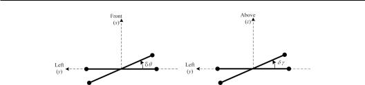
(a) Head rotation around the vertical axis (b) Head tilting around the front-backaxis
Figure 6.1 Head-turning around the vertical and front-back axes: (a) head rotation around the vertical axis; (b) head tilting around the front-back axis.
where PA is the amplitude, and k is the wave number. The interaural phase difference in pressures is calculated from Equation (6.1.1) as
L R 2kasin S cos S, |
|
(6.1.2) |
|||
or the interaural phase delay difference ITDp is given by |
|
|
|||
ITDp S, S |
|
2a |
|
|
|
|
|
c sin S cos |
S. |
(6.1.3) |
|
2 f |
When the sound source is located in the cone of confusion in Figure 1.21, sinθS cosϕS and ITDp are constant. Therefore, ITDp only is inadequate for determining the unique position of a sound source.
In Figure 6.1(a), if the head rotates around the vertical (z) axis anticlockwise with a small azimuth δθ in the horizontal (x–y) plane, ITDp becomes
ITDp S , S |
2a sin S cos S. |
(6.1.4) |
|
c |
|
Letting δθ→ 0, the variation rate or derivative of ITDp with respect to δθ is expressed as
dITDp S, S |
|
2a |
cos S cos S. |
(6.1.5) |
d |
c |
Equation (6.1.5) indicates that the variation in ITDp with head rotation is relevant to the elevation ϕS. For a given θS ≠ 90°, the magnitude of ITDp variation maximizes in the horizontal plane with ϕS = 0°. As the source elevation departs from the horizontal plane to a high or low elevation, the magnitude of variation decreases. At the top or bottom with ϕS = ±90°, ITDp is invariant against head rotation. Therefore, ITDp variation caused by head rotation provides information on vertical displacement from the horizontal plane. However, the variation in ITDp with head rotation alone does not provide enough information on up-down discrimination because of the even function characteristic of cosϕS.
As shown in Figure 6.1 (b), if the head turns around the front-back (x) axis to the left with a small angle δγ (tilting), the positions of the left and right ears become (0, acosδγ, −asinδγ) and (0, −acosδγ, asinδγ) in Cartesian coordinates, respectively. Similar to the above derivation, ITDp becomes
ITDp S, S, 2ca sin S cos S cos sin S sin . |
(6.1.6) |

Multichannel spatial surround sound 217
Letting δγ → 0, the variation rate or derivative of ITDp with respect to δγ is given by
dITDp S, S |
|
2a |
sin S. |
(6.1.7) |
d |
c |
In a horizontal plane with ϕS = 0°, ITDp is invariant against head tilting. As the source departs from the horizontal plane to a high or low elevation, the magnitude of ITDp variation with head tilting increases. Head tilting provides supplementary information on up-down discrimination because of the odd function characteristic of sinϕS. This analysis is the mathematical expression of Wallach’s hypothesis and was experimentally validated by Perrett and Noble (1997).
In the case of summing localization with multiple loudspeakers, if M loudspeakers are arranged on a spherical surface with a large radius r0>>a, then the incident wave near the origin can be approximated as a plane wave. Let (θi, ϕi) be the direction of the ith loudspeaker and Ai be the normalized amplitude or gain of the corresponding loudspeaker signal. According to Section 3.2.1, for a unit signal waveform in the frequency domain, binaural sound pressures are a linear superposition of the plane wave (far-field) pressures caused by all loudspeakers; for the arbitrary signal waveform EA(f), the following equation should be multiplied by EA(f):
|
|
M 1 |
|
|
|
|
|
|
|
P |
|
A exp |
jk |
r asin |
i |
cos |
|
|
|
L |
|
i |
|
|
0 |
i |
(6.1.8) |
||
|
|
i 0 |
|
|
|
|
|
. |
|
|
|
|
|
|
|
|
|
|
|
|
|
M 1 |
|
|
|
|
|
|
|
P |
|
A exp jk |
r asin |
i |
cos |
|
|
||
R |
|
i |
|
|
0 |
i |
|
i 0
Similar to the case of two-channel stereophonic sound in Section 2.1.1, the interaural phase delay difference is evaluated using
ITDp,SUM SUM
2 f
|
|
|
M 1 |
|
|
|
|
|
Ai sin kasin i cos i |
|
|
|
1 |
|
i 0 |
|
(6.1.9) |
|
arctan |
|
. |
||
f |
M 1 |
||||
|
|
Ai cos kasin i cos i |
|
|
|
|
|
|
|||
|
|
|
i 0 |
|
|
ITDp is the dominant cue for lateral localization at low frequencies; as such, the lateral position of the virtual source for a fixed head is found by comparing Equations (6.1.9) and (6.1.3):
|
|
|
|
M 1 |
|
|
|
|
|
|
Ai sin kasin i cos i |
|
|
sin I cos I |
|
1 |
|
i 0 |
|
(6.1.10) |
|
arctan |
|
. |
|||
ka |
M 1 |
|||||
|
|
|
Ai cos kasin i cos i |
|
|
|
|
|
|
|
|||
|
|
|
|
i 0 |
|
|

218 Spatial Sound
Equation (6.1.10) indicates that the virtual source direction generally depends on ka or frequency. At very low frequencies with ka << 1, Equation (6.1.10) can be expanded as a Taylor series of ka. If the first expansion term is retained, the equation is simplified as
M 1
Ai sin i cos i
sin I cos I i 0 M 1 . (6.1.11)
Ai
i 0
In this case, the virtual source direction is independent of ka or frequency.
If the head rotates around the vertical (z) axis anticlockwise with a small azimuth δθ, the
variation rate ITDp,SUM with δθ can also be evaluated. At very low frequencies with ka << 1, the result is
|
|
|
M 1 |
|
|
dITDp,SUM |
|
2a |
Ai cos i cos i |
|
|
i 0 |
. |
(6.1.12) |
|||
d |
c |
M 1 |
|||
|
Ai |
|
|
||
|
|
|
|
|
i 0
If ITDp variation caused by head rotation provides information on vertical displacement from a horizontal plane, then comparing Equation (6.1.12) with Equation (6.1.5) yields
M 1
Ai cos i cos i
cos I cos I i 0 M 1 . (6.1.13)
Ai
i 0
Similarly, if the head tilts around the front-back axis with a small angle δγ, the variation
rate ITDp,SUM with δγ can also be evaluated. If head tilting provides supplementary information on up-down discrimination, then comparing the result of multiple loudspeakers with
Equation (6.1.7) at very low frequencies with ka << 1 yields
M 1
Ai sin i
sin I |
i 0 |
. |
(6.1.14) |
M 1 |
|||
|
Ai |
|
|
i 0
Equations (6.1.11), (6.1.13), and (6.1.14) are a set of summing localization equations for multiple loudspeakers in a three-dimensional space.
In addition, if the head rotates around the vertical axis with an angle δθ, ITDp,SUM in Equation (6.1.9) becomes