Multichannel horizontal surround sound  199

lateral region of 54.6° < θ < 110°. This defect influences slightly and remains acceptable in sound reproduction with accompanying pictures. However, as stated in Section 1.8.3, the lateral early reflections from θ = 55° ± 20° are vital to the auditory spatial impression (especially the ASW) in a concert hall. A 5.1-channel sound with pair-wise amplitude panning fails to simulate and reproduce the spatial information of lateral reflections perfectly and therefore displays a defect in music reproduction only. This defect also reveals the limitations of using the indirect method discussed in Section 3.1 to simulate the auditory sensation of a concert hall in 5.1-channel reproduction. Further analysis of the 5.1-channel loudspeaker configuration with LS and RS loudspeakers at ±120° yields similar results (Xie, 1997). A virtual source localization experiment also validates the aforementioned analysis (Xie, 1997; Xie, 2001a; Martin et al., 1999).

The aforementioned characteristics and defects are due to the 5.1-channel loudspeaker configuration. The 5.1-channel sound was originally designed for sound reproduction with accompanying pictures; therefore, an irregular and front-biased loudspeaker configuration is used. It was not originally intended to recreate the full 360° virtual source in the horizontal plane. Using 5.1-channel sound for general reproduction (including music reproduction only) is a compromise. The analysis in this section reveals the limitation of 5.1-channel sound with pair-wise amplitude panning. Other signal panning and mixing methods are also available to recreate a virtual source in the 5.1-channel sound, and the decorrelated signal method is applicable to simulate the subjective sensation in reflective environments.

5.2.3  Global Ambisonic-like signal mixing for 5.1-channel sound

In addition to pair-wise amplitude panning, other signal panning and mixing methods have been explored for the 5.1-channel sound. Sound field or Ambisonic-like signal mixing methods similar to those discussed in Section 4.3 are suggested for recreating the virtual source in various horizontal directions, although the 5.1-channel loudspeaker configuration is inherently inappropriate for recreating a full 360° horizontal virtual source. Deriving Ambisoniclike decoding matrices or signals for irregular loudspeaker configurations based on physical and psychoacoustic criteria is complicated and sometimes difficult. Despite their complexity, some authors derived Ambisonic-like signals and mixing methods for 5.1-channel loudspeaker configurations. These methods are theoretically attractive but rarely used in practical program production.

As a general case, if M loudspeakers are arranged in a horizontal circle with regular or irregular azimuthal intervals and the azimuth of the ith loudspeaker is θi, the normalized signal amplitude of the ith loudspeaker is a linear combination of azimuthal harmonics up to the order Q,

where θS is the azimuth of the target source. In contrast to the case of a regular loudspeaker configuration given by Equation (4.3.50), the coefficients D01 i for different loudspeakers are different in the case of irregular loudspeaker configurations; as such, they cannot be identically normalized to a unit. Given the loudspeaker configuration and the order Q, the decoding matrix or loudspeaker signals are derived by searching for a set of decoding coef-

Multichannel horizontal surround sound  201

1.Criterion 1. The virtual source direction θv evaluated from the velocity localization vector given by Equation (3.2.22) should be equal to θE evaluated from the energy localization vector given by Equation (3.2.34), and θv and θE should be as close to the target source direction as possible, i.e.,

2.Criterion 2. For all target source azimuths θS or part of target source azimuths for which the accuracy of localization is important, the velocity vector magnitude rv given by Equation (3.2.29) is optimized as close to the unit as possible at low frequencies

below 0.4–0.7 kHz. The energy vector magnitude rE expressed in Equation (3.2.36) is optimized as close to the unit as possible within the midand high-frequency range of 0.7–4.0 kHz.

3.Criterion 3. The overall sound pressures P′A and overall power Pow′ in the origin should be a constant and independent from the target source azimuth θS.

For the first-order signals and if the velocity localization vector is considered only, the optimized criterion yields a set of linear equations of the decoding coefficients, which can be easily solved. In Equation (5.2.15), the amplitudes of the first-order loudspeaker signals are written as

Letting θv=θS, rv= 1, and applying the criterion of P′A = PA = 1 (i.e., the overall reproduced sound pressure in the origin is equal to the unit target sound pressure), Equations (3.2.20) and (3.2.22) yield

The left sides of the three equations above represent the normalized pressure, x, and y components of the velocity localization vector of the reproduced sound field in the origin, respectively. The right sides of the above equations represent the three corresponding physical quantities in the target sound field, respectively. Therefore, Equation (5.2.23) shows that the three physical quantities in reproduction match with those in the target sound field. Substituting Equation (5.2.22) into Equation (5.2.23) yields a linear matrix equation for the unknown coefficients:

202  Spatial Sound

where S2D = [W, X, Y]T is a 3 ×1 column matrix or vector composed of the first-order independent signals given by Equation (4.3.3), the subscript “2D” denotes the case of two-dimen- sional (horizontal) reproduction. [D2D] is an M×3 decoding matrix to be determined:

[Y2D] is a 3 × M matrix with its entries being the cosine and sine of each loudspeaker azimuth:

For M > 3, the unknown coefficients in Equation (5.2.24) can be solved from the following pseudo-inverse methods:

The solution given by Equation (5.2.27) is valid for regular and irregular loudspeaker configurations and satisfies the condition of constant-amplitude normalization given by Equation (4.3.80a). When M= 3, if the matrix [Y2D] is invertible, the solution of Equation (5.2.24) is directly obtained from the inverse matrix of [Y2D]. For regular loudspeaker configuration, the solution or loudspeaker signals expressed in Equation (5.2.27) are equivalent to Equation (4.3.15) with b = 2 and constant-amplitude normalization. For irregular loudspeaker configurations such as 5.1-channel configuration, the solution given by Equation (5.2.27) is often close to singular and thus unstable (Neukom, 2006). In this case, a slight change in loudspeaker positions or responses may influence the performance in reproduction. In addition, the following undesirable situation may occur. That is, the signal amplitude for a loudspeaker near the target source direction is large; the signal amplitude for some other loudspeakers is also large but out of phase. The destructive interference among the sound wave from all loudspeakers makes the superposed sound pressure in the origin match with that of the target source, but the overall power of all loudspeaker signals increases dramatically. Moreover, the superposed sound pressure at the off-central (off-origin) position deviates from that of the target plane wave obviously.

If the energy localization vector is considered, the optimized criteria yield a set of nonlinear equations of the unknown coefficients. Solving these equations deals with the problem of nonlinear optimization and thus is complicated. The equations are usually solved by numerical methods. The following problems may occur in solving the equations:

1.For some practical irregular loudspeaker configurations, it may only be able to satisfy the aforementioned optimized criteria partly or approximately rather than completely and exactly. In addition, it may only be able to satisfy the optimized criteria in some

Multichannel horizontal surround sound  203

target source directions rather than in all target source directions. In this case, the error in target source directions that are important for auditory perception (such as frontal directions) is considered preferentially in the optimization procedure.

2.The optimized solution depends on the optimized criteria and the measures of errors. A comprehensive measure of the overall error should be a weighted combination of the errors evaluated from the aforementioned Criteria 1 to 3. The weights are chosen in accordance with the relative importance of different errors. Different error weights lead to various results.

3.The final results of some nonlinear optimization procedures depend on the initial parameters. Inappropriate initial parameters may lead to local rather than global optimized solutions.

4.Under certain optimized criteria, two or more sets of the solution of the decoding coefficients may be available. A set of appropriate solutions should be finally identified from physical and auditory analysis or even from experience.

5.Some solutions may be nearly singular and unstable so that slight variations in parameters (such as loudspeaker azimuths) remarkably change the resultant coefficients. Such a solution is obviously inappropriate.

With these problems, deriving the decoding coefficients for irregular loudspeaker configurations becomes mathematically difficult. Despite these difficulties, some studies have derived Ambisonic-decoding coefficients and signals for irregular loudspeaker configurations, especially for the 5.1-channel configuration by using various nonlinear optimization methods.

Gerzon and Barton (1992) first investigated the solution of the decoding coefficients of second-order Ambisonic-like signals for irregular configurations with five loudspeakers. They presented their results at the 92nd Convention of the Audio Engineering Society held in Vienna and termed Vienna decoders. The azimuths of loudspeakers in Gerzon’s configuration slightly differ from those recommended by the ITU. In Gerzon’s configuration, the span angle between the left and right loudspeakers in the front was wider than that recommended by the ITU, and the span angle between a pair of surround loudspeakers was narrower than that recommended by the ITU. The ITU did not publish the standard of 5.1-channel sound when Gerzon presented his work in 1992. Gerzon outlined a method for solving decoding coefficients but did not give a detailed mathematical derivation. Many set solutions are available for the decoding coefficients. These solutions depend on some predetermined parameters that should be chosen on the basis of certain auditory localization criteria. The optimization of a velocity localization vector below 0.4 kHz and an energy localization vector at above 0.7 kHz yields two sets of decoding coefficients at low and mid-high frequencies, respectively. Accordingly, the lowand mid-high-frequency components of independent signals are individually decoded by two decoding matrices rather than a common decoding matrix and shelf filters similar to those in Figure 4.19. The overall gains of two decoding matrices are chosen to balance the timbre between low and mid-high frequencies so that the root-mean-square value of decoding coefficients at mid-high frequencies matches with that at low frequencies. This signal mixing method improves the horizontal localization performance and the stability of the front virtual source.

Craven (2003) gave the frequency-independent decoding equation for an ITU 5.1-chan- nel configuration with the 4th-order Ambisonic-like signal mixing. Decoding coefficients were derived from the cost function based on the aforementioned optimized criteria. The conjugate-gradient method was used to solve the nonlinear optimization problem. The final convergence was accelerated using the second derivatives in a Newton iteration. Craven presented the final results of (un-normalized) loudspeaker signal amplitudes or gains as shown in the following equations but did not provide the detailed mathematical derivation:

204 Spatial Sound

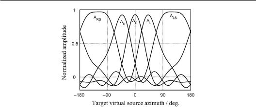
Figure 5.7 The 4th-orderAmbisonic-like signal panning curves for an ITU 5.1-channel loudspeaker configuration.

(5.2.28)

ALS 0.356 0.360cos S 0.425sin S 0.064cos2 S 0.118sin 2 S0.047 sin3 S 0.027 cos4 S 0.061sin 4 S

ARS 0.356 0.360cos S 0.425sin S 0.064cos2 S 0.118sin 2 S0.047 sin3 S 0.027 cos4 S 0.061sin 4 S

Figure 5.7 illustrates the signal panning curves of Equation (5.2.28). The amplitudes of AL, AR, ALS, and ARS signals, especially the two surround signals, are asymmetric about the axis direction of the corresponding loudspeakers. This asymmetry is adapted to an irregular loudspeaker configuration. By contrast, for regular loudspeaker configurations, the amplitudes of loudspeaker signals given by Equation (4.3.53) are even functions of the variable (θS – θi) and therefore symmetric about the axis directions of the corresponding loudspeakers. The symmetry can also be observed in the example illustrated in Figure 4.17. In addition, for a regular loudspeaker configuration, the Q-order Ambisonic reproduction requires at least (2Q + 1) or (2Q + 2) loudspeakers (Section 4.3.3). Therefore, a regular five-loudspeaker configuration is appropriate for the firstand second-order Ambisonic reproduction. Conversely, for an irregular loudspeaker configuration, higher-order azimuthal harmonic components are necessary to fit the required asymmetric polar pattern of loudspeaker signals.

Craven (2003) presented some evaluated results for loudspeaker signals given in Equation (5.2.28). Overall, the velocity vector magnitude rvis improved at the lateral direction θS = 90° and the rear direction θS =180° in comparison with those of the pair-wise amplitude panning. For example, at the rear direction θS = 180°, rv is 0.693for loudspeaker signals expressed in Equations (5.2.13) and 0.342 for pair-wise amplitude panning. This finding is due to the out- of-phase and small-amplitude AL and AR signals in Equation (5.2.28). However, the accuracy of the virtual source near θS = 50° should be further improved.

Poletti (2007)used the criterion of minimizing the overall square error between the reproduced sound pressures and target plane wave pressures to design Ambisonic signals.

Multichannel horizontal surround sound  205

A weighted combination of the power of each loudspeaker signal is used as a penalty function and added to the cost function of the square error to enhance the stability and avoid the excessive overall power of loudspeaker signals caused by an irregular loudspeaker configuration. The weights in the penalty function depend on the difference between the direction of each loudspeaker and the direction of the target source. On the basis of this method, Poletti designed a decoding equation for an ITU 5.1-channel loudspeaker configuration with the 4th- order Ambisonic-like signal mixing.

Wiggins (2007) used a Tabu search method to derive the decoding coefficients for an ITU 5.1-channel loudspeaker configuration with the 4th-order Ambisonic-like signal mixing. L (uniform) target source directions θS, l with l = 0, 1, 2… (L – 1) are chosen within the ­azimuthal region of −180° < θS ≤ 180° (or considering the left–right symmetry within the azimuthal region of −180 ° < θS ≤ 180°). Six root-mean-square (RMS) errors are evaluated:

1.Err1 is the RMS error of the reproduced sound pressure P′A(θS,,l) at the origin over the L target directions. P′A(θS,,l) is calculated from Equation (5.2.19), and the target sound pressure at the origin is normalized to a unit.

2.Err2 is the RMS error of the reproduced power Pow′(θS,,l) at the origin over the L target directions. Pow′(θS,,l) is calculated from Equation (5.2.19), and the target power is normalized to a unit.

3.Err3 is the RMS error of the velocity vector magnitude rv(θS,,l) over the L target directions. rv(θS,,l) is calculated from Equation (3.2.29), and the ideal value of rv is a unit.

4.Err4 is the RMS error of the energy vector magnitude rE(θS,,l) over the L target directions. rE(θS,,l) is calculated from Equation (3.2.36), and the ideal value of rE is a unit.

5.Err5 is the RMS error of the velocity localization vector-based azimuth θv,,l over L target directions. θv,,l is calculated from Equation (3.2.27), and the ideal value is θv,,l = θS,,l.

6.Err6 is the RMS error of the energy localization vector-based azimuth θE,,l over the L target directions. θE,,l is calculated from Equation (3.2.34), and the ideal value is

θE,,l = θS,,l.

The cost function for solving the decoding coefficients is a weighted combination of the six RMS errors:

The weights w1–w6 determine the relative contributions of each term in Equation (5.2.30). Increasing the weight of a certain term reduces the error caused by this term but at the cost of increasing the error caused by the other terms. Therefore, the weights should be chosen in accordance with certain psychoacoustic rules and the desired performance in reproduction.