
- •Preface
- •Introduction
- •1.1 Spatial coordinate systems
- •1.2 Sound fields and their physical characteristics
- •1.2.1 Free-field and sound waves generated by simple sound sources
- •1.2.2 Reflections from boundaries
- •1.2.3 Directivity of sound source radiation
- •1.2.4 Statistical analysis of acoustics in an enclosed space
- •1.2.5 Principle of sound receivers
- •1.3 Auditory system and perception
- •1.3.1 Auditory system and its functions
- •1.3.2 Hearing threshold and loudness
- •1.3.3 Masking
- •1.3.4 Critical band and auditory filter
- •1.4 Artificial head models and binaural signals
- •1.4.1 Artificial head models
- •1.4.2 Binaural signals and head-related transfer functions
- •1.5 Outline of spatial hearing
- •1.6 Localization cues for a single sound source
- •1.6.1 Interaural time difference
- •1.6.2 Interaural level difference
- •1.6.3 Cone of confusion and head movement
- •1.6.4 Spectral cues
- •1.6.5 Discussion on directional localization cues
- •1.6.6 Auditory distance perception
- •1.7 Summing localization and spatial hearing with multiple sources
- •1.7.1 Summing localization with two sound sources
- •1.7.2 The precedence effect
- •1.7.3 Spatial auditory perceptions with partially correlated and uncorrelated source signals
- •1.7.4 Auditory scene analysis and spatial hearing
- •1.7.5 Cocktail party effect
- •1.8 Room reflections and auditory spatial impression
- •1.8.1 Auditory spatial impression
- •1.8.2 Sound field-related measures and auditory spatial impression
- •1.8.3 Binaural-related measures and auditory spatial impression
- •1.9.1 Basic principle of spatial sound
- •1.9.2 Classification of spatial sound
- •1.9.3 Developments and applications of spatial sound
- •1.10 Summary
- •2.1 Basic principle of a two-channel stereophonic sound
- •2.1.1 Interchannel level difference and summing localization equation
- •2.1.2 Effect of frequency
- •2.1.3 Effect of interchannel phase difference
- •2.1.4 Virtual source created by interchannel time difference
- •2.1.5 Limitation of two-channel stereophonic sound
- •2.2.1 XY microphone pair
- •2.2.2 MS transformation and the MS microphone pair
- •2.2.3 Spaced microphone technique
- •2.2.4 Near-coincident microphone technique
- •2.2.5 Spot microphone and pan-pot technique
- •2.2.6 Discussion on microphone and signal simulation techniques for two-channel stereophonic sound
- •2.3 Upmixing and downmixing between two-channel stereophonic and mono signals
- •2.4 Two-channel stereophonic reproduction
- •2.4.1 Standard loudspeaker configuration of two-channel stereophonic sound
- •2.4.2 Influence of front-back deviation of the head
- •2.5 Summary
- •3.1 Physical and psychoacoustic principles of multichannel surround sound
- •3.2 Summing localization in multichannel horizontal surround sound
- •3.2.1 Summing localization equations for multiple horizontal loudspeakers
- •3.2.2 Analysis of the velocity and energy localization vectors of the superposed sound field
- •3.2.3 Discussion on horizontal summing localization equations
- •3.3 Multiple loudspeakers with partly correlated and low-correlated signals
- •3.4 Summary
- •4.1 Discrete quadraphone
- •4.1.1 Outline of the quadraphone
- •4.1.2 Discrete quadraphone with pair-wise amplitude panning
- •4.1.3 Discrete quadraphone with the first-order sound field signal mixing
- •4.1.4 Some discussions on discrete quadraphones
- •4.2 Other horizontal surround sounds with regular loudspeaker configurations
- •4.2.1 Six-channel reproduction with pair-wise amplitude panning
- •4.2.2 The first-order sound field signal mixing and reproduction with M ≥ 3 loudspeakers
- •4.3 Transformation of horizontal sound field signals and Ambisonics
- •4.3.1 Transformation of the first-order horizontal sound field signals
- •4.3.2 The first-order horizontal Ambisonics
- •4.3.3 The higher-order horizontal Ambisonics
- •4.3.4 Discussion and implementation of the horizontal Ambisonics
- •4.4 Summary
- •5.1 Outline of surround sounds with accompanying picture and general uses
- •5.2 5.1-Channel surround sound and its signal mixing analysis
- •5.2.1 Outline of 5.1-channel surround sound
- •5.2.2 Pair-wise amplitude panning for 5.1-channel surround sound
- •5.2.3 Global Ambisonic-like signal mixing for 5.1-channel sound
- •5.2.4 Optimization of three frontal loudspeaker signals and local Ambisonic-like signal mixing
- •5.2.5 Time panning for 5.1-channel surround sound
- •5.3 Other multichannel horizontal surround sounds
- •5.4 Low-frequency effect channel
- •5.5 Summary
- •6.1 Summing localization in multichannel spatial surround sound
- •6.1.1 Summing localization equations for spatial multiple loudspeaker configurations
- •6.1.2 Velocity and energy localization vector analysis for multichannel spatial surround sound
- •6.1.3 Discussion on spatial summing localization equations
- •6.1.4 Relationship with the horizontal summing localization equations
- •6.2 Signal mixing methods for a pair of vertical loudspeakers in the median and sagittal plane
- •6.3 Vector base amplitude panning
- •6.4 Spatial Ambisonic signal mixing and reproduction
- •6.4.1 Principle of spatial Ambisonics
- •6.4.2 Some examples of the first-order spatial Ambisonics
- •6.4.4 Recreating a top virtual source with a horizontal loudspeaker arrangement and Ambisonic signal mixing
- •6.5 Advanced multichannel spatial surround sounds and problems
- •6.5.1 Some advanced multichannel spatial surround sound techniques and systems
- •6.5.2 Object-based spatial sound
- •6.5.3 Some problems related to multichannel spatial surround sound
- •6.6 Summary
- •7.1 Basic considerations on the microphone and signal simulation techniques for multichannel sounds
- •7.2 Microphone techniques for 5.1-channel sound recording
- •7.2.1 Outline of microphone techniques for 5.1-channel sound recording
- •7.2.2 Main microphone techniques for 5.1-channel sound recording
- •7.2.3 Microphone techniques for the recording of three frontal channels
- •7.2.4 Microphone techniques for ambience recording and combination with frontal localization information recording
- •7.2.5 Stereophonic plus center channel recording
- •7.3 Microphone techniques for other multichannel sounds
- •7.3.1 Microphone techniques for other discrete multichannel sounds
- •7.3.2 Microphone techniques for Ambisonic recording
- •7.4 Simulation of localization signals for multichannel sounds
- •7.4.1 Methods of the simulation of directional localization signals
- •7.4.2 Simulation of virtual source distance and extension
- •7.4.3 Simulation of a moving virtual source
- •7.5 Simulation of reflections for stereophonic and multichannel sounds
- •7.5.1 Delay algorithms and discrete reflection simulation
- •7.5.2 IIR filter algorithm of late reverberation
- •7.5.3 FIR, hybrid FIR, and recursive filter algorithms of late reverberation
- •7.5.4 Algorithms of audio signal decorrelation
- •7.5.5 Simulation of room reflections based on physical measurement and calculation
- •7.6 Directional audio coding and multichannel sound signal synthesis
- •7.7 Summary
- •8.1 Matrix surround sound
- •8.1.1 Matrix quadraphone
- •8.1.2 Dolby Surround system
- •8.1.3 Dolby Pro-Logic decoding technique
- •8.1.4 Some developments on matrix surround sound and logic decoding techniques
- •8.2 Downmixing of multichannel sound signals
- •8.3 Upmixing of multichannel sound signals
- •8.3.1 Some considerations in upmixing
- •8.3.2 Simple upmixing methods for front-channel signals
- •8.3.3 Simple methods for Ambient component separation
- •8.3.4 Model and statistical characteristics of two-channel stereophonic signals
- •8.3.5 A scale-signal-based algorithm for upmixing
- •8.3.6 Upmixing algorithm based on principal component analysis
- •8.3.7 Algorithm based on the least mean square error for upmixing
- •8.3.8 Adaptive normalized algorithm based on the least mean square for upmixing
- •8.3.9 Some advanced upmixing algorithms
- •8.4 Summary
- •9.1 Each order approximation of ideal reproduction and Ambisonics
- •9.1.1 Each order approximation of ideal horizontal reproduction
- •9.1.2 Each order approximation of ideal three-dimensional reproduction
- •9.2 General formulation of multichannel sound field reconstruction
- •9.2.1 General formulation of multichannel sound field reconstruction in the spatial domain
- •9.2.2 Formulation of spatial-spectral domain analysis of circular secondary source array
- •9.2.3 Formulation of spatial-spectral domain analysis for a secondary source array on spherical surface
- •9.3 Spatial-spectral domain analysis and driving signals of Ambisonics
- •9.3.1 Reconstructed sound field of horizontal Ambisonics
- •9.3.2 Reconstructed sound field of spatial Ambisonics
- •9.3.3 Mixed-order Ambisonics
- •9.3.4 Near-field compensated higher-order Ambisonics
- •9.3.5 Ambisonic encoding of complex source information
- •9.3.6 Some special applications of spatial-spectral domain analysis of Ambisonics
- •9.4 Some problems related to Ambisonics
- •9.4.1 Secondary source array and stability of Ambisonics
- •9.4.2 Spatial transformation of Ambisonic sound field
- •9.5 Error analysis of Ambisonic-reconstructed sound field
- •9.5.1 Integral error of Ambisonic-reconstructed wavefront
- •9.5.2 Discrete secondary source array and spatial-spectral aliasing error in Ambisonics
- •9.6 Multichannel reconstructed sound field analysis in the spatial domain
- •9.6.1 Basic method for analysis in the spatial domain
- •9.6.2 Minimizing error in reconstructed sound field and summing localization equation
- •9.6.3 Multiple receiver position matching method and its relation to the mode-matching method
- •9.7 Listening room reflection compensation in multichannel sound reproduction
- •9.8 Microphone array for multichannel sound field signal recording
- •9.8.1 Circular microphone array for horizontal Ambisonic recording
- •9.8.2 Spherical microphone array for spatial Ambisonic recording
- •9.8.3 Discussion on microphone array recording
- •9.9 Summary
- •10.1 Basic principle and implementation of wave field synthesis
- •10.1.1 Kirchhoff–Helmholtz boundary integral and WFS
- •10.1.2 Simplification of the types of secondary sources
- •10.1.3 WFS in a horizontal plane with a linear array of secondary sources
- •10.1.4 Finite secondary source array and effect of spatial truncation
- •10.1.5 Discrete secondary source array and spatial aliasing
- •10.1.6 Some issues and related problems on WFS implementation
- •10.2 General theory of WFS
- •10.2.1 Green’s function of Helmholtz equation
- •10.2.2 General theory of three-dimensional WFS
- •10.2.3 General theory of two-dimensional WFS
- •10.2.4 Focused source in WFS
- •10.3 Analysis of WFS in the spatial-spectral domain
- •10.3.1 General formulation and analysis of WFS in the spatial-spectral domain
- •10.3.2 Analysis of the spatial aliasing in WFS
- •10.3.3 Spatial-spectral division method of WFS
- •10.4 Further discussion on sound field reconstruction
- •10.4.1 Comparison among various methods of sound field reconstruction
- •10.4.2 Further analysis of the relationship between acoustical holography and sound field reconstruction
- •10.4.3 Further analysis of the relationship between acoustical holography and Ambisonics
- •10.4.4 Comparison between WFS and Ambisonics
- •10.5 Equalization of WFS under nonideal conditions
- •10.6 Summary
- •11.1 Basic principles of binaural reproduction and virtual auditory display
- •11.1.1 Binaural recording and reproduction
- •11.1.2 Virtual auditory display
- •11.2 Acquisition of HRTFs
- •11.2.1 HRTF measurement
- •11.2.2 HRTF calculation
- •11.2.3 HRTF customization
- •11.3 Basic physical features of HRTFs
- •11.3.1 Time-domain features of far-field HRIRs
- •11.3.2 Frequency domain features of far-field HRTFs
- •11.3.3 Features of near-field HRTFs
- •11.4 HRTF-based filters for binaural synthesis
- •11.5 Spatial interpolation and decomposition of HRTFs
- •11.5.1 Directional interpolation of HRTFs
- •11.5.2 Spatial basis function decomposition and spatial sampling theorem of HRTFs
- •11.5.3 HRTF spatial interpolation and signal mixing for multichannel sound
- •11.5.4 Spectral shape basis function decomposition of HRTFs
- •11.6 Simplification of signal processing for binaural synthesis
- •11.6.1 Virtual loudspeaker-based algorithms
- •11.6.2 Basis function decomposition-based algorithms
- •11.7.1 Principle of headphone equalization
- •11.7.2 Some problems with binaural reproduction and VAD
- •11.8 Binaural reproduction through loudspeakers
- •11.8.1 Basic principle of binaural reproduction through loudspeakers
- •11.8.2 Virtual source distribution in two-front loudspeaker reproduction
- •11.8.3 Head movement and stability of virtual sources in Transaural reproduction
- •11.8.4 Timbre coloration and equalization in transaural reproduction
- •11.9 Virtual reproduction of stereophonic and multichannel surround sound
- •11.9.1 Binaural reproduction of stereophonic and multichannel sound through headphones
- •11.9.2 Stereophonic expansion and enhancement
- •11.9.3 Virtual reproduction of multichannel sound through loudspeakers
- •11.10.1 Binaural room modeling
- •11.10.2 Dynamic virtual auditory environments system
- •11.11 Summary
- •12.1 Physical analysis of binaural pressures in summing virtual source and auditory events
- •12.1.1 Evaluation of binaural pressures and localization cues
- •12.1.2 Method for summing localization analysis
- •12.1.3 Binaural pressure analysis of stereophonic and multichannel sound with amplitude panning
- •12.1.4 Analysis of summing localization with interchannel time difference
- •12.1.5 Analysis of summing localization at the off-central listening position
- •12.1.6 Analysis of interchannel correlation and spatial auditory sensations
- •12.2 Binaural auditory models and analysis of spatial sound reproduction
- •12.2.1 Analysis of lateral localization by using auditory models
- •12.2.2 Analysis of front-back and vertical localization by using a binaural auditory model
- •12.2.3 Binaural loudness models and analysis of the timbre of spatial sound reproduction
- •12.3 Binaural measurement system for assessing spatial sound reproduction
- •12.4 Summary
- •13.1 Analog audio storage and transmission
- •13.1.1 45°/45° Disk recording system
- •13.1.2 Analog magnetic tape audio recorder
- •13.1.3 Analog stereo broadcasting
- •13.2 Basic concepts of digital audio storage and transmission
- •13.3 Quantization noise and shaping
- •13.3.1 Signal-to-quantization noise ratio
- •13.3.2 Quantization noise shaping and 1-Bit DSD coding
- •13.4 Basic principle of digital audio compression and coding
- •13.4.1 Outline of digital audio compression and coding
- •13.4.2 Adaptive differential pulse-code modulation
- •13.4.3 Perceptual audio coding in the time-frequency domain
- •13.4.4 Vector quantization
- •13.4.5 Spatial audio coding
- •13.4.6 Spectral band replication
- •13.4.7 Entropy coding
- •13.4.8 Object-based audio coding
- •13.5 MPEG series of audio coding techniques and standards
- •13.5.1 MPEG-1 audio coding technique
- •13.5.2 MPEG-2 BC audio coding
- •13.5.3 MPEG-2 advanced audio coding
- •13.5.4 MPEG-4 audio coding
- •13.5.5 MPEG parametric coding of multichannel sound and unified speech and audio coding
- •13.5.6 MPEG-H 3D audio
- •13.6 Dolby series of coding techniques
- •13.6.1 Dolby digital coding technique
- •13.6.2 Some advanced Dolby coding techniques
- •13.7 DTS series of coding technique
- •13.8 MLP lossless coding technique
- •13.9 ATRAC technique
- •13.10 Audio video coding standard
- •13.11 Optical disks for audio storage
- •13.11.1 Structure, principle, and classification of optical disks
- •13.11.2 CD family and its audio formats
- •13.11.3 DVD family and its audio formats
- •13.11.4 SACD and its audio formats
- •13.11.5 BD and its audio formats
- •13.12 Digital radio and television broadcasting
- •13.12.1 Outline of digital radio and television broadcasting
- •13.12.2 Eureka-147 digital audio broadcasting
- •13.12.3 Digital radio mondiale
- •13.12.4 In-band on-channel digital audio broadcasting
- •13.12.5 Audio for digital television
- •13.13 Audio storage and transmission by personal computer
- •13.14 Summary
- •14.1 Outline of acoustic conditions and requirements for spatial sound intended for domestic reproduction
- •14.2 Acoustic consideration and design of listening rooms
- •14.3 Arrangement and characteristics of loudspeakers
- •14.3.1 Arrangement of the main loudspeakers in listening rooms
- •14.3.2 Characteristics of the main loudspeakers
- •14.3.3 Bass management and arrangement of subwoofers
- •14.4 Signal and listening level alignment
- •14.5 Standards and guidance for conditions of spatial sound reproduction
- •14.6 Headphones and binaural monitors of spatial sound reproduction
- •14.7 Acoustic conditions for cinema sound reproduction and monitoring
- •14.8 Summary
- •15.1 Outline of psychoacoustic and subjective assessment experiments
- •15.2 Contents and attributes for spatial sound assessment
- •15.3 Auditory comparison and discrimination experiment
- •15.3.1 Paradigms of auditory comparison and discrimination experiment
- •15.3.2 Examples of auditory comparison and discrimination experiment
- •15.4 Subjective assessment of small impairments in spatial sound systems
- •15.5 Subjective assessment of a spatial sound system with intermediate quality
- •15.6 Virtual source localization experiment
- •15.6.1 Basic methods for virtual source localization experiments
- •15.6.2 Preliminary analysis of the results of virtual source localization experiments
- •15.6.3 Some results of virtual source localization experiments
- •15.7 Summary
- •16.1.1 Application to commercial cinema and related problems
- •16.1.2 Applications to domestic reproduction and related problems
- •16.1.3 Applications to automobile audio
- •16.2.1 Applications to virtual reality
- •16.2.2 Applications to communication and information systems
- •16.2.3 Applications to multimedia
- •16.2.4 Applications to mobile and handheld devices
- •16.3 Applications to the scientific experiments of spatial hearing and psychoacoustics
- •16.4 Applications to sound field auralization
- •16.4.1 Auralization in room acoustics
- •16.4.2 Other applications of auralization technique
- •16.5 Applications to clinical medicine
- •16.6 Summary
- •References
- •Index

184 Spatial Sound
then the loudspeaker signals are given as
A |
A |
1 cos |
|
S |
|
Q . |
(4.3.79) |
i S |
total |
|
|
i |
|
Similar to Equation (4.3.40) for the first-order Ambisonics, for arbitrary Q-order Ambisonic signals given in Equation (4.3.53), although the virtual source direction is independent from
Atotal, Atotal determines the overall sound pressure or power in reproduction. For the constant amplitude normalization similar to Equation (4.3.41), Atotal can be obtained from the first
equation in Equation (4.3.56)
Atotal = |
1 |
. |
(4.3.80a) |
|
|||
|
M |
|
This equation is identical to the result of the first-order Ambisonics. For the constant power normalization similar to Equation (4.3.43), the following equation can be obtained:
Atotal |
|
|
|
1 |
|
. |
(4.3.80b) |
|
|
|
|
|
|||
|
|
|
Q |
|
|||
|
|
|
|
|
|
||
|
|
|
|
|
|||
|
M |
|
1 |
2 |
|
|
|
|
|
2 q |
|
|
|||
|
|
|
|
q 1 |
|
|
For κq = κ0 = 1 given in Equation (4.3.62),
Atotal |
|
1 |
. |
(4.3.81) |
|
|
|||
M |
2Q 1 |
|||
|
|
|
|
For κq expressed in Equation (4.3.77),
Atotal |
|
1 |
|
. |
(4.3.82) |
|
|
|
|||
M |
Q 1 |
|
|||
|
|
|
|
|
4.3.4 Discussion and implementation of the horizontal Ambisonics
From the point of multichannel loudspeaker signals, Ambisonics is a global amplitudebased mixing or panning method. From the point of information representation, Ambisonic encodes the spatial information of a sound field into a set of independent and universal signals, which are independent from the loudspeaker configuration in reproduction. Diverse and equivalent forms of independent signals are available. The number and configuration of loudspeakers for Ambisonic reproduction are flexible. Loudspeaker signals are derived from independent signals by decoding equations or matrices. Ambisonics can recreate the spatial information of sound field at the central listening position and up to a certain frequency limit. Therefore, Ambisonics is a universal and flexible system from the point of signal transmission and reproduction.
From the point of physics, Ambisonics is a series of systems with various orders that are based on the principle of spatial harmonics decomposition and each order approximation of the sound field. In Section 1.9.1, Ambisonics is a typical example of a gradual transition

Horizontal surround with regular loudspeaker configuration 185
from the approximate to the exact reconstruction of the target sound field. The lower-order spatial harmonics in Ambisonics represent the rough information of the spatial sound field, and the higher harmonics represent the detailed information of the spatial sound field. When the capacity of signal transmission (and storage) is limited, transmitting the information in the order from rough to detailed is reasonable. Ambisonics reduces the redundancy among the transmitted information and enables efficient use of the finite transmission capacity of the system because the independent information of the spatial sound field is extracted through spatial harmonic decomposition.
The lower-order Ambisonics can reconstruct the target sound field within a very small spatial region and limited frequency range; therefore, appropriate psychoacoustic methods should be applied to create a virtual source and other spatial auditory perceptions. The perception performance of the lower-order (e.g., the first-order) Ambisonics is limited. As the order increases, the spatial region and frequency range of the accurate transmission and reproduction of the information of the spatial sound field are extended gradually. Consequently, the spatial resolution and perceived performance of the reproduced sound field improve, and the listening region widens. However, the required number of independent signals and loudspeakers also increases as the order increases. Therefore, Ambisonics is a series of hierarchical systems in which the performance and complexity increase as the order increases. When the form of independent signals, such as the universal form of spatial harmonics given in Equation (4.3.49), is appropriately chosen, the HOA can be implemented by adding new independent signals to the lower-order Ambisonics and combining into the decoding equation. This characteristic enables the upward and downward compatibilities among different order Ambisonics. Previous studies also suggested some methods for the compatible transmission of mono, stereophonic, and first-order Ambisonic signals (Gerzon, 1985; Xie X.F., 1982).
The aforementioned features are held for horizontal and spatial Ambisonics (Section 6.4). Q-order horizontal Ambisonics involves an odd number of (2Q + 1) independent signals and requires Mmin = (2Q + 1) or more appropriately (2Q + 2) reproduction channels and loudspeakers; that is, the number of loudspeakers should be equal to or at least slightly larger than the number of independent signals. Further increasing the number of loudspeakers may improve the uniformity of the reproduced sound field but may cause new problems.
Regular horizontal loudspeaker configurations are discussed in the preceding discussion, which is true for most early domestic surround sounds. For irregular loudspeaker configurations, if loudspeakers are arranged front-back and left-right symmetrically so that each pair of loudspeakers is respectively located in two opposite directions alone the diameter of a circle, loudspeaker signals can also be derived easily. For example, the azimuths of four loudspeakers in a rectangular configuration are given as
LF 0 LB 1 180 0 RB 2 180 0 RF 3 0. |
(4.3.83) |
For the first-order Ambisonics, the signals or decoding equation of the four loudspeakers is derived similarly to that in Section 4.3.2 (Gerzon, 1985):
|
1 |
|
1 |
|
|
|
Ai S Atotal W |
|
X |
|
Y . |
(4.3.84) |
|
cos i |
sin i |
|||||
|
|
|
|
where Ai(θS) with i = 0, 1, 2, 3 denotes ALF, ALB, ARB, and ARF, respectively. When θ0 ≠ 45°, the overall power of the four loudspeaker signals is no longer a constant; instead, it depends on the target source azimuth.

186 Spatial Sound
The mathematical derivation of the decoding equation for other irregular loudspeaker configurations is complicated and may deal with the solution of nonlinear equations and numerical calculations. Moreover, some physical and psychoacoustic criteria for optimization may conflict one another; therefore, requirements from these criteria cannot be satisfied, or the solution of mathematical equations is physically inappropriate. This problem is addressed in Section 5.2.3.
In Sections 4.3.2 and 4.3.3, two methods are applied to improve the midand high-fre- quency localization performance in Ambisonic reproduction. The most effective method is to use the secondor higher-order Ambisonics. For example, a virtual source localization experiment on the Q = 1, 2, and 3-order horizontal Ambisonics indicated that the secondorder Ambisonic reproduction with six or eight loudspeakers exhibits a stable localization effect of full 360° horizontal virtual sources in the central listening position and for speech and music stimuli (Xie and Xie, 1996). This result is due to the dominant role of interaural phase delay difference and its dynamic variation with head rotation in horizontal localization (Section 1.6.5). Compared with the lower-order Ambisonics, higher-order Ambisonics further improve the perceived performance, but it is more complicated. Another method is to decode the lowand mid-to-high-frequency components with different optimizing criteria, such as the criteria of velocity localization vector and energy localization vector. In practice, a set of shelf filters is used to decode the lowand mid-to-high-frequency components of independent signals with different optimizing parameters. The crossover frequency of shelf filters is chosen on the basis of psychoacoustic consideration. Gerzon (1985) as well as Gerzon and Barton (1992) suggested a crossover frequency of 0.7 kHz for the first-order Ambisonics. Daniel et al. (1998) suggested a higher crossover frequency for the 2- and higherorder Ambisonics, such as 1.2 kHz for the second-order Ambisonics. As the order increases, the upper frequency limit for the exact reconstruction of the sound field increases. In this case, it may be unnecessary to optimize high-frequency decoding.
In Section 4.3.1, independent signals for Ambisonics have various forms corresponding to various formats of Ambisonics. Choosing W, X, and Y given in Equation (4.3.3) as the independent signals of the first-order horizontal Ambisonics is convenient. In practice, the levels of X and Y are enhanced by 3 dB to ensure a diffused field power response identical to that of M. The independent signals are written as
W W 1 X 2X 2 cos S Y 2Y 2 sin S . |
(4.3.85) |
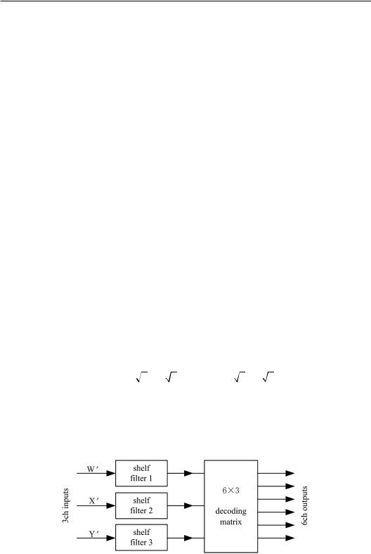
The decoding equation should be appropriately changed to make adjustments for the independent signals in Equation (4.3.85). The Ambisonic system with independent signals given by (4.3.85) is termed the first-order B-format horizontal Ambisonics (Gerzon, 1985). Figure 4.19 is the block diagram of the B-format first-order horizontal Ambisonics with six
Figure 4.19 Block diagram of the B-format first-order horizontal Ambisonics with six reproduction channels.