
- •Preface
- •Introduction
- •1.1 Spatial coordinate systems
- •1.2 Sound fields and their physical characteristics
- •1.2.1 Free-field and sound waves generated by simple sound sources
- •1.2.2 Reflections from boundaries
- •1.2.3 Directivity of sound source radiation
- •1.2.4 Statistical analysis of acoustics in an enclosed space
- •1.2.5 Principle of sound receivers
- •1.3 Auditory system and perception
- •1.3.1 Auditory system and its functions
- •1.3.2 Hearing threshold and loudness
- •1.3.3 Masking
- •1.3.4 Critical band and auditory filter
- •1.4 Artificial head models and binaural signals
- •1.4.1 Artificial head models
- •1.4.2 Binaural signals and head-related transfer functions
- •1.5 Outline of spatial hearing
- •1.6 Localization cues for a single sound source
- •1.6.1 Interaural time difference
- •1.6.2 Interaural level difference
- •1.6.3 Cone of confusion and head movement
- •1.6.4 Spectral cues
- •1.6.5 Discussion on directional localization cues
- •1.6.6 Auditory distance perception
- •1.7 Summing localization and spatial hearing with multiple sources
- •1.7.1 Summing localization with two sound sources
- •1.7.2 The precedence effect
- •1.7.3 Spatial auditory perceptions with partially correlated and uncorrelated source signals
- •1.7.4 Auditory scene analysis and spatial hearing
- •1.7.5 Cocktail party effect
- •1.8 Room reflections and auditory spatial impression
- •1.8.1 Auditory spatial impression
- •1.8.2 Sound field-related measures and auditory spatial impression
- •1.8.3 Binaural-related measures and auditory spatial impression
- •1.9.1 Basic principle of spatial sound
- •1.9.2 Classification of spatial sound
- •1.9.3 Developments and applications of spatial sound
- •1.10 Summary
- •2.1 Basic principle of a two-channel stereophonic sound
- •2.1.1 Interchannel level difference and summing localization equation
- •2.1.2 Effect of frequency
- •2.1.3 Effect of interchannel phase difference
- •2.1.4 Virtual source created by interchannel time difference
- •2.1.5 Limitation of two-channel stereophonic sound
- •2.2.1 XY microphone pair
- •2.2.2 MS transformation and the MS microphone pair
- •2.2.3 Spaced microphone technique
- •2.2.4 Near-coincident microphone technique
- •2.2.5 Spot microphone and pan-pot technique
- •2.2.6 Discussion on microphone and signal simulation techniques for two-channel stereophonic sound
- •2.3 Upmixing and downmixing between two-channel stereophonic and mono signals
- •2.4 Two-channel stereophonic reproduction
- •2.4.1 Standard loudspeaker configuration of two-channel stereophonic sound
- •2.4.2 Influence of front-back deviation of the head
- •2.5 Summary
- •3.1 Physical and psychoacoustic principles of multichannel surround sound
- •3.2 Summing localization in multichannel horizontal surround sound
- •3.2.1 Summing localization equations for multiple horizontal loudspeakers
- •3.2.2 Analysis of the velocity and energy localization vectors of the superposed sound field
- •3.2.3 Discussion on horizontal summing localization equations
- •3.3 Multiple loudspeakers with partly correlated and low-correlated signals
- •3.4 Summary
- •4.1 Discrete quadraphone
- •4.1.1 Outline of the quadraphone
- •4.1.2 Discrete quadraphone with pair-wise amplitude panning
- •4.1.3 Discrete quadraphone with the first-order sound field signal mixing
- •4.1.4 Some discussions on discrete quadraphones
- •4.2 Other horizontal surround sounds with regular loudspeaker configurations
- •4.2.1 Six-channel reproduction with pair-wise amplitude panning
- •4.2.2 The first-order sound field signal mixing and reproduction with M ≥ 3 loudspeakers
- •4.3 Transformation of horizontal sound field signals and Ambisonics
- •4.3.1 Transformation of the first-order horizontal sound field signals
- •4.3.2 The first-order horizontal Ambisonics
- •4.3.3 The higher-order horizontal Ambisonics
- •4.3.4 Discussion and implementation of the horizontal Ambisonics
- •4.4 Summary
- •5.1 Outline of surround sounds with accompanying picture and general uses
- •5.2 5.1-Channel surround sound and its signal mixing analysis
- •5.2.1 Outline of 5.1-channel surround sound
- •5.2.2 Pair-wise amplitude panning for 5.1-channel surround sound
- •5.2.3 Global Ambisonic-like signal mixing for 5.1-channel sound
- •5.2.4 Optimization of three frontal loudspeaker signals and local Ambisonic-like signal mixing
- •5.2.5 Time panning for 5.1-channel surround sound
- •5.3 Other multichannel horizontal surround sounds
- •5.4 Low-frequency effect channel
- •5.5 Summary
- •6.1 Summing localization in multichannel spatial surround sound
- •6.1.1 Summing localization equations for spatial multiple loudspeaker configurations
- •6.1.2 Velocity and energy localization vector analysis for multichannel spatial surround sound
- •6.1.3 Discussion on spatial summing localization equations
- •6.1.4 Relationship with the horizontal summing localization equations
- •6.2 Signal mixing methods for a pair of vertical loudspeakers in the median and sagittal plane
- •6.3 Vector base amplitude panning
- •6.4 Spatial Ambisonic signal mixing and reproduction
- •6.4.1 Principle of spatial Ambisonics
- •6.4.2 Some examples of the first-order spatial Ambisonics
- •6.4.4 Recreating a top virtual source with a horizontal loudspeaker arrangement and Ambisonic signal mixing
- •6.5 Advanced multichannel spatial surround sounds and problems
- •6.5.1 Some advanced multichannel spatial surround sound techniques and systems
- •6.5.2 Object-based spatial sound
- •6.5.3 Some problems related to multichannel spatial surround sound
- •6.6 Summary
- •7.1 Basic considerations on the microphone and signal simulation techniques for multichannel sounds
- •7.2 Microphone techniques for 5.1-channel sound recording
- •7.2.1 Outline of microphone techniques for 5.1-channel sound recording
- •7.2.2 Main microphone techniques for 5.1-channel sound recording
- •7.2.3 Microphone techniques for the recording of three frontal channels
- •7.2.4 Microphone techniques for ambience recording and combination with frontal localization information recording
- •7.2.5 Stereophonic plus center channel recording
- •7.3 Microphone techniques for other multichannel sounds
- •7.3.1 Microphone techniques for other discrete multichannel sounds
- •7.3.2 Microphone techniques for Ambisonic recording
- •7.4 Simulation of localization signals for multichannel sounds
- •7.4.1 Methods of the simulation of directional localization signals
- •7.4.2 Simulation of virtual source distance and extension
- •7.4.3 Simulation of a moving virtual source
- •7.5 Simulation of reflections for stereophonic and multichannel sounds
- •7.5.1 Delay algorithms and discrete reflection simulation
- •7.5.2 IIR filter algorithm of late reverberation
- •7.5.3 FIR, hybrid FIR, and recursive filter algorithms of late reverberation
- •7.5.4 Algorithms of audio signal decorrelation
- •7.5.5 Simulation of room reflections based on physical measurement and calculation
- •7.6 Directional audio coding and multichannel sound signal synthesis
- •7.7 Summary
- •8.1 Matrix surround sound
- •8.1.1 Matrix quadraphone
- •8.1.2 Dolby Surround system
- •8.1.3 Dolby Pro-Logic decoding technique
- •8.1.4 Some developments on matrix surround sound and logic decoding techniques
- •8.2 Downmixing of multichannel sound signals
- •8.3 Upmixing of multichannel sound signals
- •8.3.1 Some considerations in upmixing
- •8.3.2 Simple upmixing methods for front-channel signals
- •8.3.3 Simple methods for Ambient component separation
- •8.3.4 Model and statistical characteristics of two-channel stereophonic signals
- •8.3.5 A scale-signal-based algorithm for upmixing
- •8.3.6 Upmixing algorithm based on principal component analysis
- •8.3.7 Algorithm based on the least mean square error for upmixing
- •8.3.8 Adaptive normalized algorithm based on the least mean square for upmixing
- •8.3.9 Some advanced upmixing algorithms
- •8.4 Summary
- •9.1 Each order approximation of ideal reproduction and Ambisonics
- •9.1.1 Each order approximation of ideal horizontal reproduction
- •9.1.2 Each order approximation of ideal three-dimensional reproduction
- •9.2 General formulation of multichannel sound field reconstruction
- •9.2.1 General formulation of multichannel sound field reconstruction in the spatial domain
- •9.2.2 Formulation of spatial-spectral domain analysis of circular secondary source array
- •9.2.3 Formulation of spatial-spectral domain analysis for a secondary source array on spherical surface
- •9.3 Spatial-spectral domain analysis and driving signals of Ambisonics
- •9.3.1 Reconstructed sound field of horizontal Ambisonics
- •9.3.2 Reconstructed sound field of spatial Ambisonics
- •9.3.3 Mixed-order Ambisonics
- •9.3.4 Near-field compensated higher-order Ambisonics
- •9.3.5 Ambisonic encoding of complex source information
- •9.3.6 Some special applications of spatial-spectral domain analysis of Ambisonics
- •9.4 Some problems related to Ambisonics
- •9.4.1 Secondary source array and stability of Ambisonics
- •9.4.2 Spatial transformation of Ambisonic sound field
- •9.5 Error analysis of Ambisonic-reconstructed sound field
- •9.5.1 Integral error of Ambisonic-reconstructed wavefront
- •9.5.2 Discrete secondary source array and spatial-spectral aliasing error in Ambisonics
- •9.6 Multichannel reconstructed sound field analysis in the spatial domain
- •9.6.1 Basic method for analysis in the spatial domain
- •9.6.2 Minimizing error in reconstructed sound field and summing localization equation
- •9.6.3 Multiple receiver position matching method and its relation to the mode-matching method
- •9.7 Listening room reflection compensation in multichannel sound reproduction
- •9.8 Microphone array for multichannel sound field signal recording
- •9.8.1 Circular microphone array for horizontal Ambisonic recording
- •9.8.2 Spherical microphone array for spatial Ambisonic recording
- •9.8.3 Discussion on microphone array recording
- •9.9 Summary
- •10.1 Basic principle and implementation of wave field synthesis
- •10.1.1 Kirchhoff–Helmholtz boundary integral and WFS
- •10.1.2 Simplification of the types of secondary sources
- •10.1.3 WFS in a horizontal plane with a linear array of secondary sources
- •10.1.4 Finite secondary source array and effect of spatial truncation
- •10.1.5 Discrete secondary source array and spatial aliasing
- •10.1.6 Some issues and related problems on WFS implementation
- •10.2 General theory of WFS
- •10.2.1 Green’s function of Helmholtz equation
- •10.2.2 General theory of three-dimensional WFS
- •10.2.3 General theory of two-dimensional WFS
- •10.2.4 Focused source in WFS
- •10.3 Analysis of WFS in the spatial-spectral domain
- •10.3.1 General formulation and analysis of WFS in the spatial-spectral domain
- •10.3.2 Analysis of the spatial aliasing in WFS
- •10.3.3 Spatial-spectral division method of WFS
- •10.4 Further discussion on sound field reconstruction
- •10.4.1 Comparison among various methods of sound field reconstruction
- •10.4.2 Further analysis of the relationship between acoustical holography and sound field reconstruction
- •10.4.3 Further analysis of the relationship between acoustical holography and Ambisonics
- •10.4.4 Comparison between WFS and Ambisonics
- •10.5 Equalization of WFS under nonideal conditions
- •10.6 Summary
- •11.1 Basic principles of binaural reproduction and virtual auditory display
- •11.1.1 Binaural recording and reproduction
- •11.1.2 Virtual auditory display
- •11.2 Acquisition of HRTFs
- •11.2.1 HRTF measurement
- •11.2.2 HRTF calculation
- •11.2.3 HRTF customization
- •11.3 Basic physical features of HRTFs
- •11.3.1 Time-domain features of far-field HRIRs
- •11.3.2 Frequency domain features of far-field HRTFs
- •11.3.3 Features of near-field HRTFs
- •11.4 HRTF-based filters for binaural synthesis
- •11.5 Spatial interpolation and decomposition of HRTFs
- •11.5.1 Directional interpolation of HRTFs
- •11.5.2 Spatial basis function decomposition and spatial sampling theorem of HRTFs
- •11.5.3 HRTF spatial interpolation and signal mixing for multichannel sound
- •11.5.4 Spectral shape basis function decomposition of HRTFs
- •11.6 Simplification of signal processing for binaural synthesis
- •11.6.1 Virtual loudspeaker-based algorithms
- •11.6.2 Basis function decomposition-based algorithms
- •11.7.1 Principle of headphone equalization
- •11.7.2 Some problems with binaural reproduction and VAD
- •11.8 Binaural reproduction through loudspeakers
- •11.8.1 Basic principle of binaural reproduction through loudspeakers
- •11.8.2 Virtual source distribution in two-front loudspeaker reproduction
- •11.8.3 Head movement and stability of virtual sources in Transaural reproduction
- •11.8.4 Timbre coloration and equalization in transaural reproduction
- •11.9 Virtual reproduction of stereophonic and multichannel surround sound
- •11.9.1 Binaural reproduction of stereophonic and multichannel sound through headphones
- •11.9.2 Stereophonic expansion and enhancement
- •11.9.3 Virtual reproduction of multichannel sound through loudspeakers
- •11.10.1 Binaural room modeling
- •11.10.2 Dynamic virtual auditory environments system
- •11.11 Summary
- •12.1 Physical analysis of binaural pressures in summing virtual source and auditory events
- •12.1.1 Evaluation of binaural pressures and localization cues
- •12.1.2 Method for summing localization analysis
- •12.1.3 Binaural pressure analysis of stereophonic and multichannel sound with amplitude panning
- •12.1.4 Analysis of summing localization with interchannel time difference
- •12.1.5 Analysis of summing localization at the off-central listening position
- •12.1.6 Analysis of interchannel correlation and spatial auditory sensations
- •12.2 Binaural auditory models and analysis of spatial sound reproduction
- •12.2.1 Analysis of lateral localization by using auditory models
- •12.2.2 Analysis of front-back and vertical localization by using a binaural auditory model
- •12.2.3 Binaural loudness models and analysis of the timbre of spatial sound reproduction
- •12.3 Binaural measurement system for assessing spatial sound reproduction
- •12.4 Summary
- •13.1 Analog audio storage and transmission
- •13.1.1 45°/45° Disk recording system
- •13.1.2 Analog magnetic tape audio recorder
- •13.1.3 Analog stereo broadcasting
- •13.2 Basic concepts of digital audio storage and transmission
- •13.3 Quantization noise and shaping
- •13.3.1 Signal-to-quantization noise ratio
- •13.3.2 Quantization noise shaping and 1-Bit DSD coding
- •13.4 Basic principle of digital audio compression and coding
- •13.4.1 Outline of digital audio compression and coding
- •13.4.2 Adaptive differential pulse-code modulation
- •13.4.3 Perceptual audio coding in the time-frequency domain
- •13.4.4 Vector quantization
- •13.4.5 Spatial audio coding
- •13.4.6 Spectral band replication
- •13.4.7 Entropy coding
- •13.4.8 Object-based audio coding
- •13.5 MPEG series of audio coding techniques and standards
- •13.5.1 MPEG-1 audio coding technique
- •13.5.2 MPEG-2 BC audio coding
- •13.5.3 MPEG-2 advanced audio coding
- •13.5.4 MPEG-4 audio coding
- •13.5.5 MPEG parametric coding of multichannel sound and unified speech and audio coding
- •13.5.6 MPEG-H 3D audio
- •13.6 Dolby series of coding techniques
- •13.6.1 Dolby digital coding technique
- •13.6.2 Some advanced Dolby coding techniques
- •13.7 DTS series of coding technique
- •13.8 MLP lossless coding technique
- •13.9 ATRAC technique
- •13.10 Audio video coding standard
- •13.11 Optical disks for audio storage
- •13.11.1 Structure, principle, and classification of optical disks
- •13.11.2 CD family and its audio formats
- •13.11.3 DVD family and its audio formats
- •13.11.4 SACD and its audio formats
- •13.11.5 BD and its audio formats
- •13.12 Digital radio and television broadcasting
- •13.12.1 Outline of digital radio and television broadcasting
- •13.12.2 Eureka-147 digital audio broadcasting
- •13.12.3 Digital radio mondiale
- •13.12.4 In-band on-channel digital audio broadcasting
- •13.12.5 Audio for digital television
- •13.13 Audio storage and transmission by personal computer
- •13.14 Summary
- •14.1 Outline of acoustic conditions and requirements for spatial sound intended for domestic reproduction
- •14.2 Acoustic consideration and design of listening rooms
- •14.3 Arrangement and characteristics of loudspeakers
- •14.3.1 Arrangement of the main loudspeakers in listening rooms
- •14.3.2 Characteristics of the main loudspeakers
- •14.3.3 Bass management and arrangement of subwoofers
- •14.4 Signal and listening level alignment
- •14.5 Standards and guidance for conditions of spatial sound reproduction
- •14.6 Headphones and binaural monitors of spatial sound reproduction
- •14.7 Acoustic conditions for cinema sound reproduction and monitoring
- •14.8 Summary
- •15.1 Outline of psychoacoustic and subjective assessment experiments
- •15.2 Contents and attributes for spatial sound assessment
- •15.3 Auditory comparison and discrimination experiment
- •15.3.1 Paradigms of auditory comparison and discrimination experiment
- •15.3.2 Examples of auditory comparison and discrimination experiment
- •15.4 Subjective assessment of small impairments in spatial sound systems
- •15.5 Subjective assessment of a spatial sound system with intermediate quality
- •15.6 Virtual source localization experiment
- •15.6.1 Basic methods for virtual source localization experiments
- •15.6.2 Preliminary analysis of the results of virtual source localization experiments
- •15.6.3 Some results of virtual source localization experiments
- •15.7 Summary
- •16.1.1 Application to commercial cinema and related problems
- •16.1.2 Applications to domestic reproduction and related problems
- •16.1.3 Applications to automobile audio
- •16.2.1 Applications to virtual reality
- •16.2.2 Applications to communication and information systems
- •16.2.3 Applications to multimedia
- •16.2.4 Applications to mobile and handheld devices
- •16.3 Applications to the scientific experiments of spatial hearing and psychoacoustics
- •16.4 Applications to sound field auralization
- •16.4.1 Auralization in room acoustics
- •16.4.2 Other applications of auralization technique
- •16.5 Applications to clinical medicine
- •16.6 Summary
- •References
- •Index

Horizontal surround with regular loudspeaker configuration 153
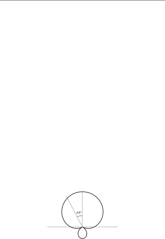
pressures and thus recreate a virtual source between loudspeakers by changing the interchannel difference (such as ICLD) between two loudspeaker signals. By contrast, a pair of LF and LB loudspeakers fail to control the interaural difference between the binaural pressures because of the front-back symmetry. The geometrical relationship of the positions of two ears and loudspeakers has been misunderstood in recreating a lateral virtual source with LF and LB loudspeakers in a quadraphone. From the point of psychoacoustics, a stable lateral virtual source cannot be recreated with a pair of lateral loudspeakers symmetrically arranged from front to back (Cooper, 1987). After the head rotates 90° to the left, the original LF and LB loudspeakers are left-right symmetrically located in the RF and left-front directions with respect to the new orientation of the head, respectively. In this case, the LF and LB loudspeakers can recreate a virtual source at the intermediate direction between two loudspeakers. This result is predicted with Equation (4.1.3).
The aforementioned analysis indicates that evaluating the virtual source direction with Equation (3.2.9) for the head oriented to the virtual source only or equally with Equation (3.2.22), derived from the velocity localization vector only, is incomplete or inappropriate. The aforementioned analysis reveals the limitation of Makita’s hypothesis. The virtual source direction should be evaluated with a combination of Equations (3.2.7) and (3.2.9), i.e., through a comprehensive analysis of the interaural phase delay difference for a fixed head and the variation in the interaural phase delay difference after head rotation.
4.1.3 Discrete quadraphone with the first-order sound field signal mixing
Similar to the XY microphone technique for two-channel stereophonic sound in Section 2.2.1, the first-order sound field signals for a discrete quadraphone can be recorded by combining the pressure and pressure-gradient microphones discussed in Section 1.2.5 (Yamamoto, 1973). Four identical combinations of pressure and pressure-gradient microphones with their main axes pointing to the horizontal LF(45°), LB(135°), RB (−135°), and RF (−45°) directions are used to capture source signals. The four microphone signals are amplified and then fed to the corresponding loudspeakers. From Equation (1.2.41), when α between the source direction and main axes of the microphones is represented with the horizontal source azimuth, the normalized amplitudes of the four microphone or loudspeaker signals are given by
A A |
A |
1 bcos |
S |
45 |
|
||
0 |
LF |
total |
|
|
|
||
A |
A |
A |
1 |
bcos |
S |
135 |
|
2 |
RB |
total |
|
|
A |
A |
A |
1 bcos |
135 |
, |
(4.1.11) |
|||||
1 |
|
LB |
|
total |
|
S |
|
|
|
||
A |
A |
|
A |
1 |
bcos |
S |
45 . |
|
|||
|
3 |
RF |
|
total |
|
|
|
|
|
where θS is the source azimuth in the original sound field or the target virtual source azimuth
in reproduction, and Atotal is a constant related to the overall gain of the system and determined by the sensitivity A′mic of microphones and the gains of amplifiers. b> 0 specifies the
directivity of microphones.
Localization theorem (Section 3.2) is applied to analyze the virtual source in reproduction (Xie X.F., 1977). At low frequencies, the virtual source position is evaluated by substituting Equations (4.1.1) and (4.1.11) into Equations (3.2.7) and (3.2.9), respectively. For a fixed head,
sin I b sin S. |
(4.1.12) |
2 |
|

154 Spatial Sound
For the head oriented to the virtual source,
tan I tan S. |
(4.1.13) |
Therefore, the perceived virtual source direction in reproduction depends on parameter b
of the microphones but is independent of the overall gain. When |
|
|
b = 2, |
(4.1.14) |
|
Equations (4.1.12) and (4.1.13) yields |
|
|
sin I sin S |
tan I tan S . |
(4.1.15) |
That is, |
|
|
I I |
S. |
(4.1.16) |
In this case, the perceived virtual source azimuth matches that of the target source within the full horizontal direction of−180° ≤ θS ≤ 180°, and the results for the head oriented to the virtual source are consistent with those of a fixed head. Moreover, Equation (3.2.29) verifies that parameter b = 2 leads to a unit velocity vector magnitude rv = 1. Therefore, a discrete quadraphone with the first-order sound field signals can theoretically recreate a full 360° horizontal virtual source at low frequencies. This feature is ideal and desirable.
The microphone with b = 2 exhibits a supercardioid directional characteristic similar to that in Figure 1.8. Figures 4.4 illustrates the two-dimensional polar pattern of a microphone
with b = 2. Atotal is normalized so that the maximal on-axis response of a microphone is a |
|
unit. Let θi represent the main axis orientation of the ith microphone. The main response |
|
(lobe) of each microphone is centered around the main axis direction θ′i |
= (θs − θi) = 0°and |
maximizes at the on-axis direction. The response magnitude decreases as | |
θ′i| increases and |
becomes null at | θ′i| = 120°. As | θ′i| further increases, the responses exhibit a negative (out- |
of-phase) rear lobe. The maximal magnitude of the rear lobe drops to −9.5 dB in comparison with that of the main lobe.
Figure 4.4 Two-dimensional polar pattern of the first-order sound field microphone with b = 2 (the maximal on-axis response is normalized to a unit).

Horizontal surround with regular loudspeaker configuration 155
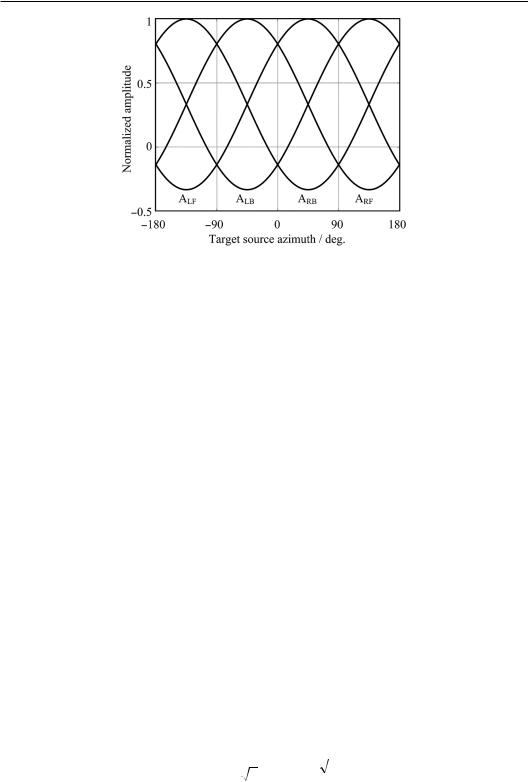
Figure 4.5 Microphone amplitude responses or the panning curve of the first-order sound field signal mixing for a quadraphone.
The pair-wise amplitude panning is a local amplitude-based panning or mixing method. In this method, a signal is mixed or panned to a pair of adjacent loudspeakers to create a virtual source between them. For a virtual source in either of the loudspeaker directions, a signal is panned to one of the loudspeakers only, and the signal of the other loudspeaker vanishes. By contrast, sound field signal mixing is an essentially global amplitude-based mixing or panning method. In this method, a signal is mixed or panned to all loudspeakers to create a virtual source except for a few target source directions. Even for a target source in a loudspeaker direction, the signal may be fed to a given loudspeaker and be spread to other loudspeakers. In other words, loudspeaker signals may encounter crosstalks. This feature distinguishes global amplitude-based mixing from local amplitude-based mixing.
Figure 4.5 illustrates the variations in four microphone amplitude responses versus a target source azimuth or the panning curve of four loudspeaker signals for the first-order sound field signal mixing. One of the four loudspeaker signals vanishes for some special target azimuths at which the angle between a given loudspeaker and the target source is 120°.Thus, the target source is exactly located in the null direction of the corresponding microphone. Even in this case, the signals of the three other loudspeakers remain. Moreover, the signal of the loudspeaker opposite to the target virtual source direction is out of phase. As stated in Section 3.2.2, this out-of-phase loudspeaker signal is necessary to ensure the velocity vector magnitude rv = 1. Therefore, from the point of psychoacoustics, the out-of-phase crosstalk signal from the opposite loudspeaker is beneficial to recreating a stable virtual source at the central listening position. However, at the off-central listening position close to the opposite loudspeakers, excessive crosstalk may cause a virtual source to collapse to the opposite loudspeaker direction.
Equation (4.1.16) is valid at very low frequencies. As frequency increases, Equation (3.2.6) should be used to evaluate the virtual source direction, and Equation (3.2.9) is applied to resolve front-back ambiguity (Xie and Liang, 1995). When Equations (4.1.1) and (4.1.11) are substituted into Equation (3.2.6), the virtual source direction for affixed head is given by
sin I |
1 |
|
|
2 |
|
|
|
|
arctan |
2 sin S tan |
ka |
. |
(4.1.17) |
||||
|
|
|||||||
|
ka |
|
|
2 |
|
|
|
|
|
|
|
|

156 Spatial Sound
When
2 |
ka |
|
, |
(4.1.18) |
|
2 |
2 |
||||
|
|
|
or
f fC |
c |
, |
(4.1.19) |
2 2a |
tan 2ka/2 0 , and sinθI possesses the same sign or polarity as sinθS. Combined with
Equation (3.2.9), θI is located in the same quadrant as θS. Equation (4.1.19) is the upper frequency limit of Equation (4.1.17). When a precorrected head radius of a′ = 1.25 × 0.0875 m to replace a in Equation (4.1.19) and when the speed of sound of c = 343 m/s is chosen, Equation (4.1.19) yields fC = 1.1 kHz.
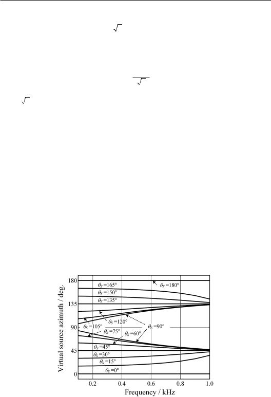
From Equations (4.1.17) and (4.1.18) and under the parameters given above, the variation in the virtual source direction with frequency for various values of θS is evaluated. Figure 4.6 illustrates the results of a target source in the left half-horizontal plane with 0° ≤ θS ≤ 180° for a fixed head. The results of the target source in the right half-horizontal plane can be derived from the left-right symmetry. Figure 4.6 indicates the following:
1. At the special source azimuths of θS = 0°,45°, 135°, and 180°, θI is independent of the frequency.
2. As frequency increases, the virtual source in the left–front quadrant with target azimuth 0° < θS < 45° and 45° < θS < 90° moves from θI = θS at low frequencies toward the direction of LF loudspeakers (45°). When frequency approaches fC as expressed in Equation (4.1.19), the virtual source is adjacent to the LF loudspeakers.
3. As frequency increases, the virtual source in the left-back quadrant with a target azimuth of 90° < θS < 135°and 135° < θS < 180° moves from θI = θS at low frequencies toward
Figure 4.6 Variation in the virtual source direction with frequency for different target azimuths in a discrete quadraphone with the first-order sound field signal mixing.