In addition, Blumlein originally used an analog circuit with the following response to equalize AS

where τm is the adjustable parameter. At low frequencies, this equalization and the inverse MS transformation also yielded stereophonic signals with ICLD only.

2.2.5  Spot microphone and pan-pot technique

Multiple spot microphones are used to capture source signals, and each microphone separately captures the signal of each source or each set of sources, resulting in multiple monosource signals. As illustrated in Figure 2.18(a), the mono signal from each spot microphone is split into two channel signals by a pan-pot. A conventional pan-pot is a dual-ganged variable resistor that controls the relative magnitude or level of the mono signal fed to the left and right channels and then leads to a different ICLD. In this case, the desired directional information of a target source is simulated or synthesized artificially. Currently, the equivalent function of a pan-pot can be easily implemented via digital signal processing.

Usually, the overall power of two channel signals is normalized to a constant (unit) to ensure equal-loudness virtual sources in different directions. Therefore, the normalized amplitudes of two signals from the pan-pot are given by

where 0° ≤ ξ ≤ 90° is a parameter. Figure 2.18(b) illustrates the variation in AL and AR with ξ. From Equation (2.1.6), for a head fixed to the frontal orientation, the direction of a low-

frequency virtual source is related to ξ as follows:

Similarly, according to Equation (2.1.10), for a head oriented to the virtual source, the direction of virtual source is evaluated by

In both cases, when ξ changes continuously from 0° to 90°, signal amplitude AR decreases continuously from 1 to 0, and AL increases continuously from 0 to 1. Accordingly, the virtual source moves continuously from −θ0 (the direction of the right loudspeaker) to θ0 (the direction of the left loudspeaker). It has AL = AR = 0.707 for ξ = 45°, i.e., a −3 dB drop off compared with the maximal amplitude of a unit value. In this case, the virtual source lies in the directly front direction of θI = 0°.

112 Spatial Sound

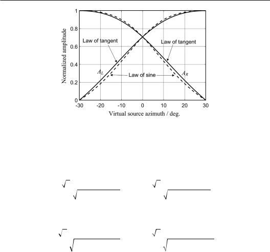
Figure 2.19 Two-channel stereophonic panning curves.

For constant-power panning, the normalized amplitudes of two channel signals can be derived from Equations (2.2.60) or (2.2.61) subjected to the condition of a constant (unit) overall power. For a head fixed to the front orientation, we have

For a head rotating to the orientation of the virtual source, we have

Equation (2.2.62) or Equation (2.2.63) gives normalized amplitudes of two channel signals as functions of a virtual source direction, i.e., signal panning function. Figure 2.19 plots the panning functions, i.e., the panning curve of the left and right channel signals for a stereophonic loudspeaker configuration with a span angle of 2θ0 = 60°. In the front and either loudspeaker directions (0°, ±30°), Equations (2.2.62) and (2.2.63) yield identical results. The two equations yield different results in other directions. However, the difference is trivial if the span angle 2θ0 between two loudspeakers does not exceed 60°.

Applying the transformation ξ = θS+ 45° with −45° ≤ θS ≤ 45°, Equation (2.2.59) becomes

This expression is consistent with Equation (2.2.11). Therefore, the nature of synthesizing two-channel stereophonic signals with pan-pot is equivalent to the artificial simulation of the signals from a coincident bidirectional XY microphone pair for a source within the effective recording range. Here, θS is the azimuth of a target source in the original sound field to be simulated rather than the direction of the perceived virtual source in reproduction shown in Equation (2.2.12).

Two-channel stereophonic sound  113

In addition to constant-power panning, two-channel signals are sometimes normalized according to the condition of constant unit amplitude, i.e., constant-amplitude panning:

The recorded signals in Equation (2.2.37) satisfy the condition of constant amplitude. The constant-amplitude and constant-power panning are relatively appropriate for reproduction in anechoic rooms and rooms with some reverberation, respectively.

In practice, the acoustic characteristics of reproduction rooms are usually frequency dependent. Some studies have introduced a frequency-dependent normalization for two channel signals according to the acoustic characteristics of a reproduction room (Laitinen et al., 2014), i.e.,

where 1 ≤ λ = λ(f, DTT) ≤ 2 is a parameter depending on frequency (band) and direct-to-total energy ratio (DTT). The DTT can be evaluated using the method in Section 1.2.4. λ =1 and

λ=2 corresponds to constant amplitude and constant-power panning, respectively. Equations (2.2.62) and (2.2.63) are derived from the stereophonic laws of sine and tan-

gent respectively. For practical music stimuli, however, the direction of the perceived virtual source may not exactly match the results of the laws of sine and tangent. Therefore, Lee and Rumsey (2013) derived the relationship between the direction of the perceived virtual source and ICLD based on the fitting of the results of a localization experiment for music stimuli and used this relationship for panning curve design.

2.2.6  Discussion on microphone and signal simulation techniques for two-channel stereophonic sound

Various microphone and signal simulation techniques for two-channel stereophonic sound are presented in the previous sections. These techniques are chosen and used flexibly according to practical requirements.

The MS, XY, and near-coincident microphone techniques are usually chosen for large orchestra recording to achieve a fused sensation in reproduction. The microphone technique and associated parameters, such as the type, directivities, distance to source (orchestra), effective recording angle of coincident microphone pairs, or various parameters of a near-coin- cident microphone pair, are chosen on the basis of practical conditions. The directivities for some coincident microphone products are adjustable and therefore convenient for practical uses.

The performance of XY and MS microphone pairs is compared in some studies (Hibbing, 1989). Although XY and MS microphone pairs are theoretically equivalent, the MS microphone pair is relatively flexible in practical use. Deriving various XY-equivalent signals from a pair of MS signals is relatively easy, freeing from the restriction on available XY microphone products with the desired directivity. At the same time, a practical directional microphone usually possesses the perfect or desired directivity below a certain frequency. As frequency increases, the main lobe of microphones usually narrows. As a result, the high-frequency output magnitude of the directional microphone decreases for an off-axis source, giving rise to timbre coloration in reproduction. This phenomenon occurs in the direct front source in XY recording, especially in an XY recording with a wide span angle between the main axis orientations of two microphones, because the source lies at the off-axis direction of two

114  Spatial Sound

microphones. This problem can be avoided in MS recording because the main axis of the M microphone always points in the front direction. Indeed, the effectiveness of the MS pair in reducing timbre coloration depends on the relative importance of the timbre of the front source at the overall stereophonic stage.

From the preceding analysis on XY coincident microphone pairs (or equivalent MS microphone pairs) and near-coincident microphone pairs, the span angle between the main axes of two microphones, effective recording range, and the span angle between two loudspeakers in reproduction are usually not coincident. The span angle between the main axes of two microphones is just a parameter related to microphone configuration. For sound sources within the effective recording range, the virtual sources in reproduction are limited or mapped to a range between two loudspeakers, when the case of outside-boundary virtual source is not considered. For many living recording stereophonic program materials, virtual source positions in reproduction are not exactly consistent with those of the actual source (such as instruments) at the original stage. However, this consistency is not vital because listeners usually do not care about the absolute positions of sound (virtual) sources in reproduction. Recreating the relative position distribution of virtual sources in reproduction is enough.

For on-site stereophonic recording, one important step is to choose the effective recording range. The effective recording range is determined by the width of source stage (span angle of source distribution with respect to microphones). A wide source stage requires a wide effective recording range. In some experiences from on-site recording, for a narrow sound stage (such as quartet), the effective recording range is chosen to be about 10% wider than the total sound stage to leave a side room (Williams and Du, 2001). However, for a wide sound stage (such as an orchestra), the effective recording range is chosen to be about 10% smaller than the sound stage to enable better resolution of the central orchestra. For an excessively wide sound stage, microphones can be placed backward at a more distant position from the sources to reduce the span angle of source distribution with respect to microphones so that all sources at the sound stage can be recorded by a pair of microphones with a smaller effective recording range. However, when the microphone pair is placed at a more distant position from the sources, the captured power of reverberation sound increases compared with that of the direct sound. In this case, a microphone pair with appropriate directivities, such as a cardioid pair in Figure 2.8(a), can be used to reduce the relative proportion of reverberation components in captured signals. Therefore, the choice of the effective recording range, the distance between a source and microphones, and the directivities and orientation of the main axes of microphones are closely related and restrained. An appropriate choice should be on the basis of practical conditions.

In some situations, stereophonic recording with a coincident or near-coincident microphone pair may not satisfy the requirement from the point of acoustics. In these cases, some additional microphones (or microphone sets) are needed. As the first example, for some music program recordings, such as solo in a concerto, the solo should be enhanced from the background of orchestral music. In this case, in addition to a coincident or near-coincident microphone pair for recording orchestral music, an individual microphone is used to capture the source signal of a solo, and the resultant signal is mixed to the two channel signals by pan-pot (for large solo instruments, such as a piano, a pair of additional microphones are needed). As a second example, for an orchestra with excessive width, instruments at two sides of the orchestra are located at a more distant distance from the coincident microphone pair and lead to a low magnitude in microphone outputs. In this case, a pair of outrigger microphones can be supplemented to the two sides to capture the source signals from the instruments at two sides of the orchestra and the outputs of an outrigger microphone pair are mixed with those of the main microphone pairs. The virtual source of the instruments at the two sides lies in the position of two loudspeakers in reproduction because of the