Chapter 2

Two-channel stereophonic sound

A two-channel stereophonic sound is the simplest and most common spatial sound technique and system. The spatial information within a certain frontal–horizontal sector (one-dimen- sional space) can be recreated on the basis of the principle of sound field approximation and psychoacoustics by using a pair of frontal loudspeakers. The two-channel stereophonic sound is considered a milestone in the developments and applications of spatial sound techniques and is still the most popular technique in use. This chapter is not intended to review the detailed history and development of the two-channel stereophonic sound. For details, readers can refer to a previous study (Xie X.F., 1981). In this chapter, the basic principles and some issues related to the applications of the two-channel stereophonic sound are presented to provide readers with sufficient background information for further discussion on multichannel surround in succeeding chapters. In Section 2.1, the basic principle of recreating spatial information by the two-channel stereophonic sound is addressed. The corresponding summing localization equations are derived, and some rules in the summing localization of a virtual source are discussed. In Section 2.2, methods for generating two-channel stereophonic signals are introduced, including various microphone recording and signal simulating techniques. In Section 2.3, the compatibility between stereophonic and mono reproduction and the problems of up/downmixing between mono and stereophonic signals are briefly discussed. In Section 2.4, some issues related to practical two-channel stereophonic reproduction, such as loudspeaker arrangement, the compensation for off-central listening position are addressed.

2.1  BASIC PRINCIPLE OF A TWO-CHANNEL STEREOPHONIC SOUND

2.1.1  Interchannel level difference and summing localization equation

The two-channel stereophonic sound is designed on the basis of the results of summing localization with two sound sources (loudspeakers) described in Section 1.7.1. In the late 1950s and beginning of the 1960s, the principle of two-channel stereophonic sound was reanalyzed by some researches (Clack et al., 1957; Leakey, 1959; Bauer, 1961a; Makita, 1962; Mertens, 1965).

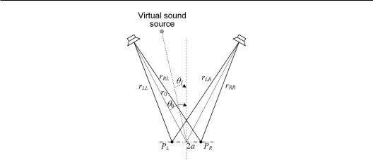
In Figure 2.1, a pair of loudspeakers are arranged symmetrically in the front of the listener with azimuths θL = θ0 and θR = −θ0. The two loudspeaker signals in the frequency domain are EL and ER (stereophonic signals are usually denoted as notation L and R, whereas frequencydomain signals are denoted as notation E in this book). Two identical loudspeaker signals with different amplitudes are written as

Two-channel stereophonic sound  73

where k = 2π f/c is the wave number, and c = 343 m/s is the speed of sound, and

denote the distances from the loudspeaker to the ipsilateral (near) and contralateral (far) ears, respectively. At a distance of r0 >> a, if incident waves from loudspeakers are represented as a spherical wave rather than approximated as plane waves, AL and AR in Equation (2.1.2) are substituted with AL/4πr0 and AR/4πr0, respectively. Even in this case, the resultant localization equation is identical to that derived by the approximation of a plane wave. In Equations (2.1.2) and (2.1.3), the common phase factor exp(−jkr0) represents the linear delay caused by the sound propagation from each loudspeaker to the origin and can be omitted. Omitting this phase factor is equivalent to supplementing an initial linear phase exp(jkr0) to the complex-valued strength Qp of the point source or loudspeakers mentioned above. This manipulation is also equivalent to a normalization that makes the transfer coefficient from the loudspeaker signal to the pressure amplitude of the free-field plane wave at the origin to be a unit. Then, the interaural phase difference is calculated as

The subscript “SUM” in the two equations represents the case of summing localization with two loudspeakers. As stated in Section 1.6.5, the interaural phase delay difference is considered a dominant cue for azimuthal localization at low frequencies. A comparison between the combined ITDp,SUM in Equation (2.1.4b) and the single-source ITDp derived from prior auditory experiences [Equation (1.6.1)] enables the determination of the azimuthal position θI of the summing virtual source as

At low frequencies with ka << 1, Equation (2.1.5) can be expanded as a Taylor series of ka (or ka sinθ0). If the first expansion term is retained, the equation can be simplified as

This expression is the virtual source localization equation for the two-channel stereophonic sound, i.e., the famous stereophonic law of sine. This law demonstrates that the spatial position θI of the summing virtual source is completely determined by the amplitude ratio (AL/AR) between the two loudspeaker signals and the half-span angle θ0 between the two loudspeakers with respect to the listener, but it is irrelevant to frequency and head radius. For an average head radius with a = 0.0875 m, Equation (2.1.6) is quite effective below 0.7 kHz.

74 Spatial Sound

Thus, Equation (2.1.6) suggests the following:

1.When AL and AR are identical, sinθI is zero, indicating that the summing virtual source is positioned at the midpoint between two loudspeakers.

2.When AL is larger than AR, sinθI is positive, meaning that the summing virtual source is positioned close to the left loudspeaker.

3.When AL is far larger than AR, sinθI is approximately equal to sinθ0, indicating that the summing virtual source is positioned at the left loudspeaker.

4. Similar results are obtained when AR is larger than AL because of the left-right symmetry in configuration.

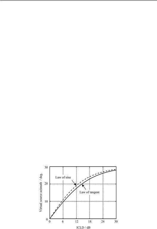
In Equation (2.1.6), θ0 = 30° or 2θ0 = 60°(standard stereophonic loudspeaker configuration) is substituted, and the relationship between the position of the virtual source and the interchannel level difference (ICLD) between loudspeaker signals denoted by d = 20 log10(AL/AR) dB is illustrated in Figure 2.2. In Figure 2.2, θI varies continuously from 0° to approximately 30°as d increases from 0 dB to +30 dB. This finding is consistent with the results of the virtual source localization experiment with two stereophonic loudspeakers.

Some remarks on summing localization with two stereophonic loudspeakers and the stereophonic law of sine are as follows:

1. The stereophonic law of sine is based on the principle of the summing localization of two sound sources. In stereophonic localization, ITDp,SUM encoded in the superposed binaural pressures is used by the auditory system to identify the position of the virtual source at low frequencies. ITDp,SUM is controlled by the ICLD. This finding indicates that transformation occurs from the ICLD at the two loudspeaker signals to ITDp,SUM at the binaural pressures. The ICLD regarding the loudspeaker signals should not be confused with the interaural level difference (ILD) at the two ears (introduced in Section 1.6.2).

2. The approach of creating localization cues by adjusting the ICLD is invalid above 1.5 kHz for two-channel stereophonic reproduction because the superposed binaural pressures contain only the localization cue of ITDp, which is an effective cue below 1.5 kHz. For wideband stimuli containing low-frequency components below 1.5 kHz,

Figure 2.2 Relationship between the position of the virtual source and the interchannel level difference between the loudspeaker signals calculated from the stereophonic laws of sine and tangent, respectively.

Two-channel stereophonic sound  75

creating a virtual source by using ICLD is still valid because of the dominant role of ITDp in azimuthal localization at low frequencies.

3. An anticlockwise spherical coordinate system with respect to the head center is employed in this book. If the clockwise spherical coordinate system is used, a negative sign should be supplemented to the sine law in Equation (2.1.6).

The law of sine is derived under the assumption that a listener’s head is fixed to the front orientation. When the listener’s head rotates around the vertical axis with an azimuth δθ (δθ > 0 represents an anticlockwise rotation to the left, and δθ < 0 denotes a clockwise rotation to the right), the distances from two loudspeakers to two ears in Figure 2.1 become

Similar to the derivation from Equation (2.1.1) to (2.1.4), the interaural phase delay difference becomes

The azimuth δθ of the rotation represents the virtual source direction with respect to the fixed coordinate, i.e., ˆI , by choosing the azimuth δθ of rotation so that the listener is oriented to the virtual source direction and the interaural phase delay difference ITDp,SUM given by Equation (2.1.8) consequently vanishes. Here, the notation θˆI is used to denote the azimuth of the virtual source because the result of the head’s rotation may be different from that of the fixed head orientation. When ITDp,SUM = 0 is substituted in Equation (2.1.8), the following equation is obtained:

At low frequencies with ka << 1, Equation (2.1.9) can be expanded as a Taylor series of ka. If only the first expansion term is retained, the virtual source azimuth is determined in accordance with the law of tangent

For an average head radius, Equation (2.1.10) is quite effective below 0.7 kHz. Makita (1962) supposed that the perceived virtual source direction in the superposed sound field is consistent with the inner normal direction (opposite to the direction of the medium velocity) of the superposed wavefront at the receiver position. Equation (2.1.10) can also be derived from Makita’s hypothesis (Section 3.2.2). Actually, Makita’s hypothesis is equivalent to that of the rotation of the listener’s head to the orientation of the virtual source.

The results calculated from Equation (2.1.10) are presented in Figure 2.2. In particular, the span angle between two loudspeakers is also 2θ0 = 60°. The results of Equation (2.1.10) are similar to those of Equation (2.1.6) because tanθ ≈ sinθ for θ ≤ 30°. Therefore, for loudspeaker configuration with the span angle 2θ0 ≤ 60°, the perceived virtual source direction is relatively stable during head rotation. In practice, Equations (2.1.6) and (2.1.10) are