
- •Preface
- •Introduction
- •1.1 Spatial coordinate systems
- •1.2 Sound fields and their physical characteristics
- •1.2.1 Free-field and sound waves generated by simple sound sources
- •1.2.2 Reflections from boundaries
- •1.2.3 Directivity of sound source radiation
- •1.2.4 Statistical analysis of acoustics in an enclosed space
- •1.2.5 Principle of sound receivers
- •1.3 Auditory system and perception
- •1.3.1 Auditory system and its functions
- •1.3.2 Hearing threshold and loudness
- •1.3.3 Masking
- •1.3.4 Critical band and auditory filter
- •1.4 Artificial head models and binaural signals
- •1.4.1 Artificial head models
- •1.4.2 Binaural signals and head-related transfer functions
- •1.5 Outline of spatial hearing
- •1.6 Localization cues for a single sound source
- •1.6.1 Interaural time difference
- •1.6.2 Interaural level difference
- •1.6.3 Cone of confusion and head movement
- •1.6.4 Spectral cues
- •1.6.5 Discussion on directional localization cues
- •1.6.6 Auditory distance perception
- •1.7 Summing localization and spatial hearing with multiple sources
- •1.7.1 Summing localization with two sound sources
- •1.7.2 The precedence effect
- •1.7.3 Spatial auditory perceptions with partially correlated and uncorrelated source signals
- •1.7.4 Auditory scene analysis and spatial hearing
- •1.7.5 Cocktail party effect
- •1.8 Room reflections and auditory spatial impression
- •1.8.1 Auditory spatial impression
- •1.8.2 Sound field-related measures and auditory spatial impression
- •1.8.3 Binaural-related measures and auditory spatial impression
- •1.9.1 Basic principle of spatial sound
- •1.9.2 Classification of spatial sound
- •1.9.3 Developments and applications of spatial sound
- •1.10 Summary
- •2.1 Basic principle of a two-channel stereophonic sound
- •2.1.1 Interchannel level difference and summing localization equation
- •2.1.2 Effect of frequency
- •2.1.3 Effect of interchannel phase difference
- •2.1.4 Virtual source created by interchannel time difference
- •2.1.5 Limitation of two-channel stereophonic sound
- •2.2.1 XY microphone pair
- •2.2.2 MS transformation and the MS microphone pair
- •2.2.3 Spaced microphone technique
- •2.2.4 Near-coincident microphone technique
- •2.2.5 Spot microphone and pan-pot technique
- •2.2.6 Discussion on microphone and signal simulation techniques for two-channel stereophonic sound
- •2.3 Upmixing and downmixing between two-channel stereophonic and mono signals
- •2.4 Two-channel stereophonic reproduction
- •2.4.1 Standard loudspeaker configuration of two-channel stereophonic sound
- •2.4.2 Influence of front-back deviation of the head
- •2.5 Summary
- •3.1 Physical and psychoacoustic principles of multichannel surround sound
- •3.2 Summing localization in multichannel horizontal surround sound
- •3.2.1 Summing localization equations for multiple horizontal loudspeakers
- •3.2.2 Analysis of the velocity and energy localization vectors of the superposed sound field
- •3.2.3 Discussion on horizontal summing localization equations
- •3.3 Multiple loudspeakers with partly correlated and low-correlated signals
- •3.4 Summary
- •4.1 Discrete quadraphone
- •4.1.1 Outline of the quadraphone
- •4.1.2 Discrete quadraphone with pair-wise amplitude panning
- •4.1.3 Discrete quadraphone with the first-order sound field signal mixing
- •4.1.4 Some discussions on discrete quadraphones
- •4.2 Other horizontal surround sounds with regular loudspeaker configurations
- •4.2.1 Six-channel reproduction with pair-wise amplitude panning
- •4.2.2 The first-order sound field signal mixing and reproduction with M ≥ 3 loudspeakers
- •4.3 Transformation of horizontal sound field signals and Ambisonics
- •4.3.1 Transformation of the first-order horizontal sound field signals
- •4.3.2 The first-order horizontal Ambisonics
- •4.3.3 The higher-order horizontal Ambisonics
- •4.3.4 Discussion and implementation of the horizontal Ambisonics
- •4.4 Summary
- •5.1 Outline of surround sounds with accompanying picture and general uses
- •5.2 5.1-Channel surround sound and its signal mixing analysis
- •5.2.1 Outline of 5.1-channel surround sound
- •5.2.2 Pair-wise amplitude panning for 5.1-channel surround sound
- •5.2.3 Global Ambisonic-like signal mixing for 5.1-channel sound
- •5.2.4 Optimization of three frontal loudspeaker signals and local Ambisonic-like signal mixing
- •5.2.5 Time panning for 5.1-channel surround sound
- •5.3 Other multichannel horizontal surround sounds
- •5.4 Low-frequency effect channel
- •5.5 Summary
- •6.1 Summing localization in multichannel spatial surround sound
- •6.1.1 Summing localization equations for spatial multiple loudspeaker configurations
- •6.1.2 Velocity and energy localization vector analysis for multichannel spatial surround sound
- •6.1.3 Discussion on spatial summing localization equations
- •6.1.4 Relationship with the horizontal summing localization equations
- •6.2 Signal mixing methods for a pair of vertical loudspeakers in the median and sagittal plane
- •6.3 Vector base amplitude panning
- •6.4 Spatial Ambisonic signal mixing and reproduction
- •6.4.1 Principle of spatial Ambisonics
- •6.4.2 Some examples of the first-order spatial Ambisonics
- •6.4.4 Recreating a top virtual source with a horizontal loudspeaker arrangement and Ambisonic signal mixing
- •6.5 Advanced multichannel spatial surround sounds and problems
- •6.5.1 Some advanced multichannel spatial surround sound techniques and systems
- •6.5.2 Object-based spatial sound
- •6.5.3 Some problems related to multichannel spatial surround sound
- •6.6 Summary
- •7.1 Basic considerations on the microphone and signal simulation techniques for multichannel sounds
- •7.2 Microphone techniques for 5.1-channel sound recording
- •7.2.1 Outline of microphone techniques for 5.1-channel sound recording
- •7.2.2 Main microphone techniques for 5.1-channel sound recording
- •7.2.3 Microphone techniques for the recording of three frontal channels
- •7.2.4 Microphone techniques for ambience recording and combination with frontal localization information recording
- •7.2.5 Stereophonic plus center channel recording
- •7.3 Microphone techniques for other multichannel sounds
- •7.3.1 Microphone techniques for other discrete multichannel sounds
- •7.3.2 Microphone techniques for Ambisonic recording
- •7.4 Simulation of localization signals for multichannel sounds
- •7.4.1 Methods of the simulation of directional localization signals
- •7.4.2 Simulation of virtual source distance and extension
- •7.4.3 Simulation of a moving virtual source
- •7.5 Simulation of reflections for stereophonic and multichannel sounds
- •7.5.1 Delay algorithms and discrete reflection simulation
- •7.5.2 IIR filter algorithm of late reverberation
- •7.5.3 FIR, hybrid FIR, and recursive filter algorithms of late reverberation
- •7.5.4 Algorithms of audio signal decorrelation
- •7.5.5 Simulation of room reflections based on physical measurement and calculation
- •7.6 Directional audio coding and multichannel sound signal synthesis
- •7.7 Summary
- •8.1 Matrix surround sound
- •8.1.1 Matrix quadraphone
- •8.1.2 Dolby Surround system
- •8.1.3 Dolby Pro-Logic decoding technique
- •8.1.4 Some developments on matrix surround sound and logic decoding techniques
- •8.2 Downmixing of multichannel sound signals
- •8.3 Upmixing of multichannel sound signals
- •8.3.1 Some considerations in upmixing
- •8.3.2 Simple upmixing methods for front-channel signals
- •8.3.3 Simple methods for Ambient component separation
- •8.3.4 Model and statistical characteristics of two-channel stereophonic signals
- •8.3.5 A scale-signal-based algorithm for upmixing
- •8.3.6 Upmixing algorithm based on principal component analysis
- •8.3.7 Algorithm based on the least mean square error for upmixing
- •8.3.8 Adaptive normalized algorithm based on the least mean square for upmixing
- •8.3.9 Some advanced upmixing algorithms
- •8.4 Summary
- •9.1 Each order approximation of ideal reproduction and Ambisonics
- •9.1.1 Each order approximation of ideal horizontal reproduction
- •9.1.2 Each order approximation of ideal three-dimensional reproduction
- •9.2 General formulation of multichannel sound field reconstruction
- •9.2.1 General formulation of multichannel sound field reconstruction in the spatial domain
- •9.2.2 Formulation of spatial-spectral domain analysis of circular secondary source array
- •9.2.3 Formulation of spatial-spectral domain analysis for a secondary source array on spherical surface
- •9.3 Spatial-spectral domain analysis and driving signals of Ambisonics
- •9.3.1 Reconstructed sound field of horizontal Ambisonics
- •9.3.2 Reconstructed sound field of spatial Ambisonics
- •9.3.3 Mixed-order Ambisonics
- •9.3.4 Near-field compensated higher-order Ambisonics
- •9.3.5 Ambisonic encoding of complex source information
- •9.3.6 Some special applications of spatial-spectral domain analysis of Ambisonics
- •9.4 Some problems related to Ambisonics
- •9.4.1 Secondary source array and stability of Ambisonics
- •9.4.2 Spatial transformation of Ambisonic sound field
- •9.5 Error analysis of Ambisonic-reconstructed sound field
- •9.5.1 Integral error of Ambisonic-reconstructed wavefront
- •9.5.2 Discrete secondary source array and spatial-spectral aliasing error in Ambisonics
- •9.6 Multichannel reconstructed sound field analysis in the spatial domain
- •9.6.1 Basic method for analysis in the spatial domain
- •9.6.2 Minimizing error in reconstructed sound field and summing localization equation
- •9.6.3 Multiple receiver position matching method and its relation to the mode-matching method
- •9.7 Listening room reflection compensation in multichannel sound reproduction
- •9.8 Microphone array for multichannel sound field signal recording
- •9.8.1 Circular microphone array for horizontal Ambisonic recording
- •9.8.2 Spherical microphone array for spatial Ambisonic recording
- •9.8.3 Discussion on microphone array recording
- •9.9 Summary
- •10.1 Basic principle and implementation of wave field synthesis
- •10.1.1 Kirchhoff–Helmholtz boundary integral and WFS
- •10.1.2 Simplification of the types of secondary sources
- •10.1.3 WFS in a horizontal plane with a linear array of secondary sources
- •10.1.4 Finite secondary source array and effect of spatial truncation
- •10.1.5 Discrete secondary source array and spatial aliasing
- •10.1.6 Some issues and related problems on WFS implementation
- •10.2 General theory of WFS
- •10.2.1 Green’s function of Helmholtz equation
- •10.2.2 General theory of three-dimensional WFS
- •10.2.3 General theory of two-dimensional WFS
- •10.2.4 Focused source in WFS
- •10.3 Analysis of WFS in the spatial-spectral domain
- •10.3.1 General formulation and analysis of WFS in the spatial-spectral domain
- •10.3.2 Analysis of the spatial aliasing in WFS
- •10.3.3 Spatial-spectral division method of WFS
- •10.4 Further discussion on sound field reconstruction
- •10.4.1 Comparison among various methods of sound field reconstruction
- •10.4.2 Further analysis of the relationship between acoustical holography and sound field reconstruction
- •10.4.3 Further analysis of the relationship between acoustical holography and Ambisonics
- •10.4.4 Comparison between WFS and Ambisonics
- •10.5 Equalization of WFS under nonideal conditions
- •10.6 Summary
- •11.1 Basic principles of binaural reproduction and virtual auditory display
- •11.1.1 Binaural recording and reproduction
- •11.1.2 Virtual auditory display
- •11.2 Acquisition of HRTFs
- •11.2.1 HRTF measurement
- •11.2.2 HRTF calculation
- •11.2.3 HRTF customization
- •11.3 Basic physical features of HRTFs
- •11.3.1 Time-domain features of far-field HRIRs
- •11.3.2 Frequency domain features of far-field HRTFs
- •11.3.3 Features of near-field HRTFs
- •11.4 HRTF-based filters for binaural synthesis
- •11.5 Spatial interpolation and decomposition of HRTFs
- •11.5.1 Directional interpolation of HRTFs
- •11.5.2 Spatial basis function decomposition and spatial sampling theorem of HRTFs
- •11.5.3 HRTF spatial interpolation and signal mixing for multichannel sound
- •11.5.4 Spectral shape basis function decomposition of HRTFs
- •11.6 Simplification of signal processing for binaural synthesis
- •11.6.1 Virtual loudspeaker-based algorithms
- •11.6.2 Basis function decomposition-based algorithms
- •11.7.1 Principle of headphone equalization
- •11.7.2 Some problems with binaural reproduction and VAD
- •11.8 Binaural reproduction through loudspeakers
- •11.8.1 Basic principle of binaural reproduction through loudspeakers
- •11.8.2 Virtual source distribution in two-front loudspeaker reproduction
- •11.8.3 Head movement and stability of virtual sources in Transaural reproduction
- •11.8.4 Timbre coloration and equalization in transaural reproduction
- •11.9 Virtual reproduction of stereophonic and multichannel surround sound
- •11.9.1 Binaural reproduction of stereophonic and multichannel sound through headphones
- •11.9.2 Stereophonic expansion and enhancement
- •11.9.3 Virtual reproduction of multichannel sound through loudspeakers
- •11.10.1 Binaural room modeling
- •11.10.2 Dynamic virtual auditory environments system
- •11.11 Summary
- •12.1 Physical analysis of binaural pressures in summing virtual source and auditory events
- •12.1.1 Evaluation of binaural pressures and localization cues
- •12.1.2 Method for summing localization analysis
- •12.1.3 Binaural pressure analysis of stereophonic and multichannel sound with amplitude panning
- •12.1.4 Analysis of summing localization with interchannel time difference
- •12.1.5 Analysis of summing localization at the off-central listening position
- •12.1.6 Analysis of interchannel correlation and spatial auditory sensations
- •12.2 Binaural auditory models and analysis of spatial sound reproduction
- •12.2.1 Analysis of lateral localization by using auditory models
- •12.2.2 Analysis of front-back and vertical localization by using a binaural auditory model
- •12.2.3 Binaural loudness models and analysis of the timbre of spatial sound reproduction
- •12.3 Binaural measurement system for assessing spatial sound reproduction
- •12.4 Summary
- •13.1 Analog audio storage and transmission
- •13.1.1 45°/45° Disk recording system
- •13.1.2 Analog magnetic tape audio recorder
- •13.1.3 Analog stereo broadcasting
- •13.2 Basic concepts of digital audio storage and transmission
- •13.3 Quantization noise and shaping
- •13.3.1 Signal-to-quantization noise ratio
- •13.3.2 Quantization noise shaping and 1-Bit DSD coding
- •13.4 Basic principle of digital audio compression and coding
- •13.4.1 Outline of digital audio compression and coding
- •13.4.2 Adaptive differential pulse-code modulation
- •13.4.3 Perceptual audio coding in the time-frequency domain
- •13.4.4 Vector quantization
- •13.4.5 Spatial audio coding
- •13.4.6 Spectral band replication
- •13.4.7 Entropy coding
- •13.4.8 Object-based audio coding
- •13.5 MPEG series of audio coding techniques and standards
- •13.5.1 MPEG-1 audio coding technique
- •13.5.2 MPEG-2 BC audio coding
- •13.5.3 MPEG-2 advanced audio coding
- •13.5.4 MPEG-4 audio coding
- •13.5.5 MPEG parametric coding of multichannel sound and unified speech and audio coding
- •13.5.6 MPEG-H 3D audio
- •13.6 Dolby series of coding techniques
- •13.6.1 Dolby digital coding technique
- •13.6.2 Some advanced Dolby coding techniques
- •13.7 DTS series of coding technique
- •13.8 MLP lossless coding technique
- •13.9 ATRAC technique
- •13.10 Audio video coding standard
- •13.11 Optical disks for audio storage
- •13.11.1 Structure, principle, and classification of optical disks
- •13.11.2 CD family and its audio formats
- •13.11.3 DVD family and its audio formats
- •13.11.4 SACD and its audio formats
- •13.11.5 BD and its audio formats
- •13.12 Digital radio and television broadcasting
- •13.12.1 Outline of digital radio and television broadcasting
- •13.12.2 Eureka-147 digital audio broadcasting
- •13.12.3 Digital radio mondiale
- •13.12.4 In-band on-channel digital audio broadcasting
- •13.12.5 Audio for digital television
- •13.13 Audio storage and transmission by personal computer
- •13.14 Summary
- •14.1 Outline of acoustic conditions and requirements for spatial sound intended for domestic reproduction
- •14.2 Acoustic consideration and design of listening rooms
- •14.3 Arrangement and characteristics of loudspeakers
- •14.3.1 Arrangement of the main loudspeakers in listening rooms
- •14.3.2 Characteristics of the main loudspeakers
- •14.3.3 Bass management and arrangement of subwoofers
- •14.4 Signal and listening level alignment
- •14.5 Standards and guidance for conditions of spatial sound reproduction
- •14.6 Headphones and binaural monitors of spatial sound reproduction
- •14.7 Acoustic conditions for cinema sound reproduction and monitoring
- •14.8 Summary
- •15.1 Outline of psychoacoustic and subjective assessment experiments
- •15.2 Contents and attributes for spatial sound assessment
- •15.3 Auditory comparison and discrimination experiment
- •15.3.1 Paradigms of auditory comparison and discrimination experiment
- •15.3.2 Examples of auditory comparison and discrimination experiment
- •15.4 Subjective assessment of small impairments in spatial sound systems
- •15.5 Subjective assessment of a spatial sound system with intermediate quality
- •15.6 Virtual source localization experiment
- •15.6.1 Basic methods for virtual source localization experiments
- •15.6.2 Preliminary analysis of the results of virtual source localization experiments
- •15.6.3 Some results of virtual source localization experiments
- •15.7 Summary
- •16.1.1 Application to commercial cinema and related problems
- •16.1.2 Applications to domestic reproduction and related problems
- •16.1.3 Applications to automobile audio
- •16.2.1 Applications to virtual reality
- •16.2.2 Applications to communication and information systems
- •16.2.3 Applications to multimedia
- •16.2.4 Applications to mobile and handheld devices
- •16.3 Applications to the scientific experiments of spatial hearing and psychoacoustics
- •16.4 Applications to sound field auralization
- •16.4.1 Auralization in room acoustics
- •16.4.2 Other applications of auralization technique
- •16.5 Applications to clinical medicine
- •16.6 Summary
- •References
- •Index

Storage and transmission of spatial sound signals 637
component, along with the time-varying directional parameter, can be transmitted as audio stream. Ambient components mainly contain nondirectional information. Because the spatial resolution of human hearing to ambient components is relatively low, they can be handled by lower-order Ambisonics to improve the coding efficiency. However, because the Ambisonic representation or signals of ambient components may be highly correlated, the spatial unmasking of quantization noise may occur after decoding. Similar to the MS stereo coding in Section 13.4.5, the Ambisonic representation is decorrelated by transforming it to a different spatial domain for perceptual coding to avoid this problem.
The decoding of Ambisonic signals is an inverse course of coding. Based on Ambisonic data from the USAC 3D core decoding, decorrelated ambient components are first transformed to the HOA representation. The HOA representation of predominant components is also resynthesized from the coded data. The HOA representations of predominant and ambient components are then combined to form HOA-independent signals. According to the practical loudspeaker configuration, HOA-independent signals are linearly decoded into loudspeaker signals. A matrix that preserves the constant power (energy) is used in decoding.
4.SAOC-3D decoding and rendering (Murtaza et al., 2015)
MPEG-H 3D Audio also supports parametrically coded channel signals and audio objects, e.g., an extended spatial audio object coding called SAOC-3D. In comparison with the original SAOC in Section 13.5.5, the SAOC-3D is extended in the following aspects.
•SAOC-3D in principle supports an arbitrary number of downmixing channels, while original SAOC supports a two-channel downmixing at most.
•SAOC-3D supports the direct decoding/rendering to multichannel outputs for arbitrary loudspeaker configurations, including the enhanced decorrelation to output signals. SAOC only support by using a MPEG surround as a rendering engine.
•Some SAOC tools, such as residual coding, are unnecessary and thus omitted in MPEG-H 3D Audio.
5.Binaural rendering
The mixed outputs in Figure 13.23 are for loudspeaker reproduction. They can be converted to signals for headphone presentation by binaural synthesis in Section 11.9.1. That is, the signal intended for each loudspeaker is convolved with a pair of binaural room impulse responses and then mixed to simulate transmission from loudspeakers to two ears in a listening room. Binaural rendering is vital in mobile devices.
6.Loudness and dynamic range control
7.Some loudness normalization and dynamic range information are embedded into the MPEG-H 3D Audio bit stream for loudness and dynamic range control in the decoder.
Subjective experiments indicated that MPEG-H 3D Audio exhibits an excellent quality at a bit rate of 1.2 Mbit/s or 512 kbit/s and shows good quality at a bit rate of 256 kbit/s. MPEG-H 3D Audio with a lower bit rate is being developed.
13.6 DOLBY SERIES OF CODING TECHNIQUES
Since the 1980s, Dolby Laboratories has developed a series of digital audio compression and coding techniques. These techniques have been widely used. However, the details of some of these techniques have not been published. This section outlines the basic principle of these techniques that have been published.

638 Spatial Sound
13.6.1 Dolby digital coding technique
The Dolby AC-1 developed in the early time is a stereophonic coding technique. It uses adaptive delta modulation (ADM) and combines with analog compounding. It is not a perceptual coding technique. The Dolby AC-2 developed in the 1980s is a coding technique for stereophonic and multichannel sound. It is a perceptual coding technique that consists of four single-channel coders/decoders (Fielder and Robinson, 1995; Brandenburg and Bosi, 1997).
Dolby Digital (AC-3) is a multichannel audio coding technique introduced in 1991. It was originally intended for 35 mm film soundtrack in a commercial cinema and subsequently specified as the audio coding standard of HDTV in USA. It has also been used widely for audio coding in DVD-Video (Davis, 1993; Davis and Todd, 1994; Todd et al., 1994; ETSI TS 102 366 V1.4.1, 2017; ATSC standard Doc.A52, 2012). Dolby Digital supports the sampling frequencies of 32, 44.1, and 48 kHz. It allows 5.1-channel coding (and mono, stereophonic, and threeand four-channel coding) with a bit rate ranging from 32 kbit/s to 640 kbit/s. A typical bit rate for 5.1-channel coding is 384 kbit/s. At this bit rate, Dolby Digital provides a good perceived audio quality (ITU-R Doc.10/51-E, 1995; Wüstenhagen et al., 1998; Gaston and Sanders, 2008).
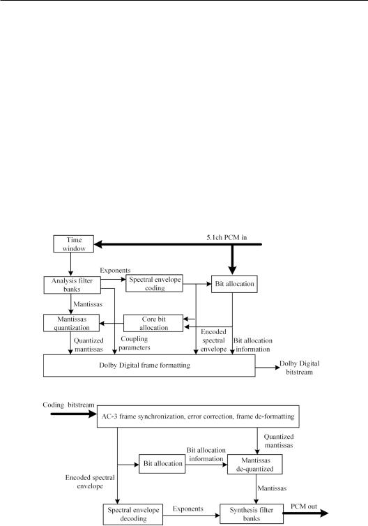
Figure 13.24 (a) illustrates the block diagram of Dolby Digital coding. After a time window, PCM input samples are transformed into time-frequency coefficients by analyzing filter
(a) Coding
(a) Decoding
Figure 13.24 Block diagram of Dolby Digital coding/decoding (a) Coding; (b) Decoding (adapted from ETSI TS 102 366 V1.4.1, 2017).

Storage and transmission of spatial sound signals 639
bands. Coefficients are normalized so that their maximal absolute magnitudes do not exceed 1. Each normalized coefficient is represented by a binary exponent and a mantissa and subsequently coded. For example, the exponent for a 16-bit binary number 0.0010 1100 0011 0001, which represents the number of “0” after the decimal point, is 2 in the decimal system or 10 in the binary system; and the mantissa is 10 1100 0011 0001 in the binary system. Binary exponents represent a rough variation in the spectral envelop and the binary mantissas represent the detail variations in the spectra. In a coder, the core bit allocation for mantissas is determined by a spectral envelope and a psychoacoustic model. The final stream involves the coded audio data, synchronous data, bitstream information, and additional data.
Figure 13.24 (b) shows the block diagram of Dolby Digital decoding. Decoding is an inverse course of coding. Various data are extracted. Mantissas are de-quantized according to bit allocation information. Spectral coefficients are reconstructed from exponents and mantissas from which PCM signals are restored using synthesis filter bands.
Some technical details of Dolby Digital coding/decoding are outlined as follows:
1.Analysis filter bands
Analysis filter bands are implemented by MDCT. The size of MDCT determines the time-frequency resolution. Dolby Digital dynamically chooses the size of MDCT. The PCM input is underground 8 kHz high-pass filters, and high-frequency energy is estimated. Stationary and transient signals are detected by comparing the resultant highfrequency energy with a pre-determined threshold.
Stationary signals require a higher-frequency resolution; therefore, MDCT with a long window (512 samples) is used. Each PCM block is overlapped by 50% with its two neighbors to avoid theartifacts caused by the abrupt transition between the border of two adjacent blocks; that is, 512 audio samples for MDCT are constructed by taking 256 samples from the previous block and 256 samples from the current block. The 512-point MDCT yields 256 spectral coefficients because of the odd symmetric relation in Equation (13.4.7). A Kaiser–Bessel window is used to improve the frequency selectivity and reduce the influence of the block border. At a sampling frequency of 48 kHz, the frequency and time resolutions of MDCT with a long window are 187.5 Hz and 5.33 ms. Transient signals require a high time resolution; therefore, MDCT with a short window (256 samples) is used. Each PCM block is also overlapped by 50% with its two neighbors. The 256-point MDCT yields 128 spectral coefficients. At a sampling frequency of 48 kHz, the frequency and time resolutions of MDCT with a short window are 375 Hz and 2.67 ms.
2.Exponent coding strategy
The exponents of spectral coefficients represent the rough variation in spectra. Dolby Digital coding allows a range of exponent values from 0 to 24 (in the decimal system). Spectral coefficients with an exponent value more than 24 (or the corresponding spectral coefficients less than 2−24) are set to 24. A differential coding is used to code the exponent within a block. The first exponent of a full-bandwidth channel (or lowfrequency effect, LFE channel) is coded with a 4-bit absolute value, corresponding to a variation from 0 to 15. Successive exponents at the ascending frequency are differentially coded and represented by one of five possible values ±2, ±1, and 0 corresponding to ±12, ±6, and 0 dB variation in magnitude, respectively. Differential exponents are combined into groups in the block. According to the bit rate and required frequency
resolution, grouping is formed by one of three exponent coding strategies, namely, D15, D25, and D45 modes, where the index “5” denotes five quantization levels of differential exponents, and index “1,” “2,” or “3” denotes the number of spectral coefficients that

640 Spatial Sound
share the same differential exponent. For example, in the D15 mode, three spectral coefficients are combined into a group, each spectral coefficient requires a differential exponent, and each differential exponent can take one of the five possible values. Therefore, there are 5 × 5 × 5 = 125 variations in differential exponents in D15 strategy. In this case, 7 bits is needed to code these variations, or 2.33 bit is required to code a differential exponent. Similar, in D25 and D45strategies, 2.17 and 0.58 bits are respectively needed to a differential exponent. The bit rate and frequency resolution descend in the order of D15, D25, and D45. The Dolby Digital coder chooses an optimal exponent coding strategy for each audio block. For stationary signals, a set of differential exponents can be shared by six MDCT blocks at most.
3.Mantissa quantization and adaptive bit allocation
As stated, Dolby Digital uses a spectral envelop and a psychoacoustic model to determine the core bit allocation for mantissa coding. In contrast to other coding methods (such as MPEG-1 layers I/II), Dolby Digital coder employs a forward-backward- adaptive psychoacoustic model. The decoder also includes a core backward-adaptive model. Core bit allocation uses a psychoacoustic model based on certain assumptions on the masking properties of signals. Some parameters of the model are also transmitted by the data stream. Therefore, the actual psychoacoustic model in a decoder can be adjusted by the coder. The coder can perform an ideal bit allocation based on a complicated but accurate psychoacoustic model and compares the results with the core bit allocation. If core bit allocation can better match the ideal bit allocation by changing some parameters, the coder does so and finishes the bit allocation. Otherwise, the coder sends some information to the decoder.
4.Channel coupling and re-matrixing
At a very low bit rate, the aforementioned compression and coding algorithms may not satisfy the bit rate requirement. In this case, spectral coefficients at high frequencies are combined into a single coupling channel to transmission. The coupling channel is formed by a vector summation of the spectral coefficients from all channels in coupling. This process is an extension of intensity stereo coding in Section 13.4.5. Channel coupling is based on the psychoacoustic principles that low-frequency ITD dominates lateral localization; at a high frequency, only the energy envelop contributes to localization. Dolby Digital decomposes signals into 18 subband components and applies the channel coupling above some subbands. Similar to original channels, spectral coefficients in the coupling channel are represented by binary exponents and a mantissa and coded. The coder calculates the powers of original signals and coupled signal. The resultant power ratio between the original signal and the coupled signal is evaluated for each input channel and each subband and transmitted as side information parameters. The decoder distributes the coupling channel signal to the output channels according to the side information parameters.
In re-matrixing, MS coding for a pair of channels with high correlation is used. It is applied to stereophonic signal coding. Its principle is outlined in Section 13.4.5.
In addition to the aforementioned technical details, Dolby Digital possesses some user features.
1.Loudness control
The level of dialog varies in different programs. Switching between different programs directly causes a variation in perceived loudness. Dolby Digital stream includes a code for dialog level normalization, which enables users to set the gain in reproduction according to the required level.