Storage and transmission of spatial sound signals  615

13.4.3  Perceptual audio coding in the time-frequency domain

Perceptual audio coding utilizes the redundancy in the perceptual domain to compress audio signals and is a lossy coding method (Brandenburg and Bosi, 1997). The masking effect in Section 1.3.3 is the psychoacoustic basis for perceptual audio coding. Section 13.3.1 indicates that mapping the continuous amplitude of a signal to finite discreate values leads to quantization­ noise. In the absence of noise shaping, signal-to-quantization-noise ratio increases as the quantization bit increases. A larger quantization bit is needed to obtain high signal-to-quantization-noise ratio. However, quantization noise is not always audible because of the masking effect. If the level of quantization noise is below the threshold of a masking curve (pattern), the quantization noise is inaudible. If the level of a signal is below the hearing threshold or below the threshold of the masking curve, the signal is also inaudible. The above psychoacoustic principles are applicable to perceptual audio coding.

Because masking is related to the time-frequency resolution of human hearing, time domain signals should be transformed to time-frequency domain signals prior to perceptual coding. Transformation has two types. They are similar in nature but different in time-frequency resolution. In practical coding, appropriate transformations and related parameters should be chosen so that time-frequency resolution meets the requirement of auditory perception.

The first type of transformation uses an analysis filter bands to decompose time domain signals into subband components. The bandwidth of subband filters can be uniform or nonuniform. Filters with a uniform bandwidth are relatively simple, but filters with a nonuniform bandwidth can be adapted to the frequency resolution of human auditory. Generally, subband filters exhibit higher time resolution and lower frequency resolution. According to Shannon–Nyquist temporal sampling theorem (Oppenheim et al., 1999), each subband component can be downconverted into a baseband and then subsampled at a sampling frequency not less than twice the bandwidth of the subband.The original signal can be restored by first upsampling and upconverting the baseband representation of each subband component and combining the components of all subbands by using a synthesis filter bank. Ideally, analysis filters should have abrupt transition characteristics between the passband and the stopband to avoid the frequency domain overlap in the restored signal. In addition, the analysis filters should have linear-phase characteristics. Filters with such kind of characteristics are difficult to be implemented. In practice, the bandwidth of signals is often divided into K uniform subbands, where K is the power of 2. Then, analysis filtering is implemented by K quadrature mirror filters (QMF). Although the outputs of quadrature mirror filters overlap at the boundaries between the subbands, overlapping components are cancelled in synthesis filtering, and the original signal is restored. A polyphase quadrature mirror filter (PQMF) band is often used in practical subband coding. For MPEG-1 Layer I and Layer II coding in Section 13.5.1, a PQMF bands is used to divide the time domain input into 32 uniform subband components. An analysis filter bands with a critical bandwidth is used for MPEG-1 Layer III coding.

In the second type of transformation, the discrete time samples of the input signal are divided into block or frames with an appropriate length, and short-term discrete orthogonal transform is used to convert each block of time samples into spectral coefficients in the transform domain (such as in the frequency domain or more strictly in the time-frequency domain). Generally, various short-term discrete orthogonal transforms exhibit higher-­frequency resolution and lower time resolution. A well-known short-term discrete orthogonal transform is the short-term Fourier transform (STFT) in Equation (8.3.15). However, modified discrete cosine transform (MDCT) is often used in spatial sound signal coding, such as Dolby Digital coding described in Section 13.6.1. The advantage of MDCT is that the power of a signal is dominated by the preceding spectral components, which are beneficial to signal compression. In addition to STFT and MDCT, other short-term discrete orthogonaltransforms, which yield the coefficients in the transform domain, are applicable to audio coding.

Storage and transmission of spatial sound signals  617

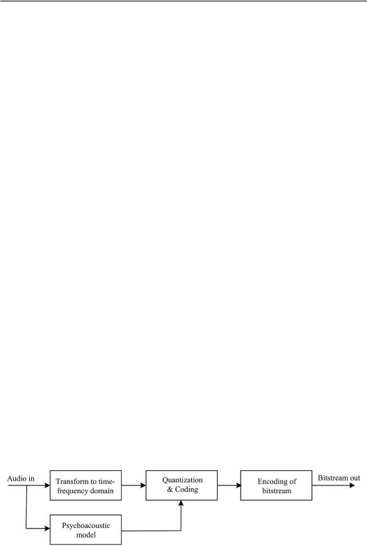
as using STFT) or directly evaluated from the result of stage (1). The resultant power spectra are analyzed by a psychoacoustic model inputted to the time-frequency domain.

3.The subband or spectral components of input signals are quantized and coded. Different

subband components or spectral coefficients Ex(n′, k) are quantized with different bits. Given the available bit rate, the algorithms of dynamic bit allocation are often used. According to the short-term power spectra evaluated in stage (2) and certain psychoacoustic models, available bits are allocated to each subband component or spectral coefficients (set) to optimize the final perceived performance.

4.The quantized data are organized into frames and then assembled into the bit stream.

In addition to the quantized and coded samples E′x(n′, k), bit stream involves some side information, such as bit allocation information for reconstructing a signal in decoding.

A decoder reconstructs the signal from the bit stream of coded signals. Decoding is an inverse course of coding (Figure 13.14). The subband components or spectral coefficients of each frame are extracted from the bit stream from which PCM audio signals are reconstructed.

Quantization, dynamic bit allocation, and coding have various algorithms. The performance of these algorithms, such as computational cost, compression ratio, and perceived effect, varies. Dynamic bit allocation strategies in audio coding have two kinds. In forwardadaptive allocation, allocation is performed in the coder, and information is included in the bit stream. An advantage of forward-adaptive allocation is that the psychoacoustic model is only included in the coder. A revision of the psychoacoustic model does not influence the design of the decoder. A disadvantage is that some bit resources are needed to convey the allocation information to the decoder. In backward-adaptive allocation, bit allocation information in the decoder is derived from the coded audio data, and the transmission of bit allocation information is not needed. Backward-adaptive allocation has a higher transmission efficiency, but it consumes the computational resource of the decoder. In addition, the psychoacoustic model in the decoder cannot be easily improved when it is applied.

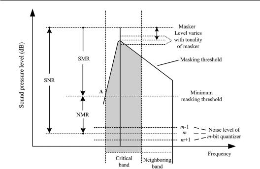
Psychoacoustic models simulate the perception of human hearing to sound. They are essential for perceptual audio coding, especially dynamic bit allocation. Various psychoacoustic models with different accuracies and complicities exist. The quantitative analysis and simulation of the masking effects are the cores of various psychoacoustic models related to audio coding. In many cases, SNRQ in each subband (critical band) is calculated from the shortterm power spectral level and given quantization bits for each frame (sampling block) of input signals. The larger the quantization bits are, the larger SNRQ will be. According to the psychoacoustic pattern of masking, the signal-to-masking-ratio SMR in each subband, which is the difference between power spectral level of signal and minimum masking threshold, is calculated. The noise-masking ratio in each subband is determined using the following formula:

NMR> 0 means that quantization noise is audible. Figure 13.15 illustrates the relationship among NMR, SMR, and SNRQ. For a given the overall bit rate, dynamic bit allocation, which is usually implemented by iterative algorithm, minimizes the overall NMR across all subbands. In addition, signal components with a level lower than the hearing threshold is inaudible. They are not coded or coded with lower bits.

Masking pattern models are needed to calculate SMR. These patterns depend on the components of stimuli (tonal or nontonal components). Many models in audio coding detect tonality in signals (such as local maximum in the spectrum or spectral flatness measure) to

618 Spatial Sound

Figure 13.15 Relationship of NMR, SMR, and SNRQ (Noll, 1997, with the permission of IEEE).

determine the range and amount of masking. In addition, the effect of the critical bandwidth component of a masker is not limited to a single critical band, but it is also distributed to other bands. The spreading function describes masking across several critical bands to simulate the masking response of the entire basilar membrane. The effects of maskers in several critical bands should be considered in the calculation of the overall masking threshold.

13.4.4 Vector quantization

Scalar quantization is discussed in the preceding sections in which each sample (or each differential sample) of the input signal is quantized and coded. Vector quantization (VQ) assembles some scalar data into a set according to a certain rule. Each set can be regarded as a vector and can be quantized jointly in a vector space (Gersho and Gray, 1992; Furui, 2000). VQ maximizes the statistical correlation between the components of the vector and compresses the data with less loss of information. As a lossy coding technique, VQ is widely used in speech coding and sometimes used in audio coding.

If the data of K scalar inputs ex0, ex1…exK constitute a K-dimensional vector ex = [ex0, ex1… exK], and the set {ex} of all K-dimensional vectors constitutes a K-dimensional Euclid space. The Euclid space is divided into L subspaces that do not intersect. Each subspace is approximately represented by a vector eyl. The set {eyl} of L representative vectors eyl (l = 0, 1… L − 1) is termed a code book. The number L of representative vectors in a code book is called the length of a code book. Various divisions of subspaces or choices of the code book constitute different vector quantizers.

For an arbitrary input vector ex, a vector quantizer first determines the subspace in which ex belongs to and then represents ex by a corresponding vector eyl. Therefore, the nature of VQ is to map the arbitrary vector ex in a K-dimensional Euclid space into a finite set {eyl} of L representative vectors.