46  Spatial Sound

independent of the source distance in the far field. However, it varies considerably as the source distance changes within the range of 1.0 m (i.e., in the near field) for a sound source outside the median plane, especially within the range of 0.5 m. ILD is irrelevant to source properties because it is defined as the ratio between the sound pressures in the two ears. Therefore, the near-field ILD is a cue for absolute distance estimation. The pressure spectrum in each ear also changes with the source distance in the near field, which potentially serves as another distance cue. These distance-dependent cues are described by near-field HRTFs. Near-field HRTFs are used to render a virtual source at various distances in a virtual auditory display (Chapter 11). However, this method is reliable only within a target source distance of 1.0 m.

Reflections in an enclosed space are effective cues for distance estimation (Nielsen, 1993). In Equation (1.2.25), the direct-to-reverberant energy ratio is inversely proportional to the square of distance. Therefore, it can be used as a distance cue, although a real reflected sound field may deviate from the diffuse sound field. Equation (1.2.25) is derived on the basis of this ratio. Bronkhorst and Houtgast (1999) indicated that a simple model based on a modified direct-to-reverberant energy ratio can accurately predict the auditory distance perception in rooms. In stereophonic and multichannel sound program production, the perceived distance is often controlled by the direct-to-reverberant energy ratio in program signals. Frequencydependent boundary absorption modifies the power spectra of reflections, and the proportion of the reflected power increases as the sound source distance increases. Thus, the power spectra of binaural pressures vary with the sound source distance. This finding also provides information for auditory distance perception.

In summary, auditory distance perception is derived from the comprehensive analyses of multiple cues. Although distance estimation has recently received increasing attention, knowledge regarding its detailed mechanism remains incomplete.

1.7  SUMMING LOCALIZATION AND SPATIAL HEARING WITH MULTIPLE SOURCES

The localization of multiple sound sources, as the localization of a single sound source presented in Section 1.6, is another important aspect of spatial hearing (Blauert, 1997). Under a specific situation, the auditory system may perceive a sound coming from a spatial position where no real sound source exists when two or more sound sources simultaneously radiate correlated sounds. Such kind of an illusory or phantom sound source, also called virtual sound source (shortened as virtual source) or virtual sound image (shortened as sound image), results from the summing localization of multiple sound sources. In summing localization, the sound pressure in each ear is a linear combination of the pressures generated by multiple sound sources. The auditory system then automatically compares the localization cues, such as ITD and ILD, encoded in binaural sound pressures with the stored patterns derived from prior experiences with a single sound source. If the cues in binaural sound pressures successfully match the pattern of a single sound source at a given spatial position, then a convincing virtual sound source at that position is perceived. However, this case is not always true. Some experimental results of summing localization remain incompletely interpreted. Overall, summing localization with multiple sound sources is a spatial auditory event that should be explained with the psychoacoustic principle (Guan, 1995).

Under some situations, multiple sources may result in other spatial auditory events. For example, in the case of the precedence effect described in Section 1.7.2, a listener perceives sounds as though they come from one of the real sources regardless of the presence of other sound sources. When two or more sound sources simultaneously radiate partially correlated

48 Spatial Sound

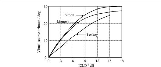
Figure 1.26 Virtual source localization experiments on loudspeaker signals with ICLD. (redrawn on the basis of the results of Leakey 1960, Mertens 1965, and Simonson 1984 and adopted from Wittek and Theile 2002).

may also be included in the results. Figure 1.26 illustrates the experimental results of a virtual source position that varies with the ICLD of loudspeaker signals obtained by Leakey (1960), Mertens (1965), and Simonson (1984). A standard angle span 2θ0 = 60° (or near 60°) between two loudspeakers was chosen in their experiments. Speech signals were used in the experiments of Leakey and Simonson. The noise signal centered at 1.1 kHz was used by Mertens. In addition, the displacements of the virtual source in the baseline were determined in some experiments. Here, they are converted to the azimuths of the virtual source.

In the same loudspeaker configuration shown in Figure 1.25, if a signal and its delayed version are fed into two loudspeakers, a virtual source moves toward the direction of the loudspeaker with the leading signal. When the interchannel time difference (ICTD) between two loudspeaker signals exceeds a certain upper limit, the virtual source moves to the direction of the loudspeaker. This result is held for impulse-like signals or some other signals with transient characteristics, such as click, speech, and music signals. However, the ICTD cannot be utilized effectively for low-frequency steady signals.

The ICTD required to position the virtual sound source to either of the loudspeakers varies considerably in different experiments and usually depends on the type of signals. It differs from several hundreds of microseconds (μs) to slightly more than 1 millisecond (ms) in most cases. Figure 1.27 illustrates the experimental results of the virtual source position varying with the ICTD obtained by Leakey (1960), Mertens (1965), and Simonson (1984). The conditions of experiments are similar to those mentioned above, but the signal used by Mertens was random noise. ICLD and ICTD are the level and time differences between two loudspeaker signals, respectively. They should not be confused with the ILD and ITD discussed in Section 1.6, which describes the level and time differences between the pressures or signals in the two ears and serve as cues for directional localization.

For some transient signals (rather than all signals), a trading effect exists between ICLD and ICTD. This effect has been experimentally investigated, but results have some differences depending on the type of signals (Leakey, 1959; Mertens, 1965; Blauert, 1997). The general tendency is summarized as follows. For loudspeaker signals with ICLD and ICTD, the movement of a virtual source enhances when the individual effects of ICLD and ICTD are consistent, and the movement of the virtual source becomes cancelled when the individual effects of ICLD and ICTD are opposite. Figure 1.28 illustrates the results of Mertens; that is, trading curves between ICLD and ICTD for the virtual source at θI = 0° and ±30°. The loudspeakers

Sound field, spatial hearing, and sound reproduction 49

Figure 1.27 Results of virtual source localization experiments for loudspeaker signals with ICTD. (redrawn on the basis of the results of Leakey 1960, Mertens 1965, Simonson 1984 and adopted from Wittek and Theile 2002.)

Figure 1.28 Trading curve between ICLD and ICTD. (redrawn on the basis of the data of Mertens, 1965 and adopted from Williams, 2013.)

are arranged at azimuths ±30°, and the signal is a Gaussian burst of white noise. The curves in Figure 1.28 are left-right symmetric. All combinations of ICTD and ICLD in each curve yield the same azimuth perception (i.e., 0°, −30°, or 30°).

As is indicated in Section 2.1 and Chapter 12, stereophonic loudspeaker signals with ICLD only results in appropriate low-frequency ITDp in the superposed sound pressures in the two ears. In addition, the ILD caused by loudspeaker signals with ICLD only is small below the frequency of 1.5 kHz, which is qualitatively consistent with the case of an actual sound source. The auditory system determines the position of a virtual source based on the comparison between the resultant ITDp and the patterns stored from previous experiences on real sound sources because ITDp dominates the lateral localization. The method of recreating a