42  Spatial Sound

the incident sound except the first one. Hence, the resonance model supports the idea that the spectral cue provided by the pinna is a directional localization cue.

Numerous psychoacoustic experiments have been devoted to exploring the localization cue encoded in spectral features. However, no general quantitative relationship between spectral features and sound source positions has been found because of the complexity and individuality of the shape and dimension of the pinna and the head. Blauert (1997) used narrow-band noise to investigate directional localization in the median plane. Experimental results show that the perceived position of a sound source is determined by the directional frequency band in the ear canal pressures regardless of the real sound source position; that is, the perceived position of a sound source is always located in specific directions, where the frequency of the spectral peak in the ear canal pressure caused by a wide-band sound coincides with the center frequency of the narrow-band noise. Hence, peaks in the ear canal pressure caused by the head and the pinna are important in localization (Middlebrooks et al., 1989).

However, some researchers argued that the spectral notch, especially the lowest frequency notch caused by the pinna (called the pinna notch), is more important for localization in the median plane and even for vertical localization outside the median plane (Hebrank and Wright, 1974; Butler and Belendiuk, 1977; Bloom, 1977; Kulkarni, 1997; Han, 1994). In front of the median plane, the center frequency of the pinna notch varies with elevation in the range of 5 or 6 kHz to about 12 or 13 kHz. This variation is due to the interaction of the incident sound arriving from different elevations to the different parts of the pinna. As a result, different diffraction and reflection delays occur relative to the direct sound. Thus, shifting frequency notch provides vertical localization information. Moore et al. (1989) found that shifting in the central frequency of the exquisitely narrow notch can be easily perceived although hearing is usually more sensitive to the spectral peak.

Other researchers contended that both peaks and notches (Watkins, 1978) or spectral profiles are important in localization (Middlebrooks, 1992). Algazi et al. (2001b) suggested that the change in the ipsilateral spectra below 3 kHz caused by the scattering and reflection of the torso, especially the shoulder, provides vertical localization information for a sound source outside the median plane.

In brief, the spectral feature caused by the diffraction and reflection of an anatomical structure, such as the head and pinna, is an important and individualized localization cue. Although a clarified and quantitative relationship between the spectral feature and the direction of a sound source is far less complete, one’s own spectral feature can be used to localize a sound source.

1.6.5  Discussion on directional localization cues

In summary, directional localization cues can be classified as follows:

1. For frequencies approximately below 1.5 kHz, the ITD derived from ITDp is the dominant cue for lateral localization.

2. Above the frequency of 1.5 kHz, ILD and ITD derived from the interaural envelope delay difference (ITDe) contribute to lateral localization. As frequency increases (approximately above 4–5 kHz), ILD gradually becomes dominant.

3. A spectral cue is important for localization. In particular, above frequencies of 5–6 kHz, a spectral cue introduced by the pinna is essential for the vertical localization and disambiguation of front–back confusion.

4. The dynamic cue introduced by the slight turning of the head is helpful in resolving front–back ambiguity and vertical localization.

Sound field, spatial hearing, and sound reproduction  43

The aforementioned directional localization cues except the dynamic cue can be evaluated from HRTFs. Therefore, HRTFs include the major directional localization cues. These localization cues are individually dependent because of the unique characteristics of anatomical structures and dimensions. The auditory system determines the position of a sound source based on a comparison between the obtained cues and patterns stored from prior experiences. However, even for the same individual, anatomical structures and dimensions vary with time, especially from childhood into adulthood albeit slowly. Therefore, a comparison with prior experiences may be a self-adaptive process, and the high-level neural system can automatically modify stored patterns by using auditory experiences.

Different kinds of localization cues work in different frequency ranges and contribute differently to localization. For sinusoidal or narrow-band stimuli, only the localization cues existing in the frequency range of the stimuli are available; hence, the resultant localization accuracy is likely to be frequency dependent. Mills (1958) investigated localization accuracy in the horizontal plane by using sinusoidal stimuli. He showed that localization accuracy is frequency dependent, and the highest accuracy is θS = 1° in front of the horizontal plane (θS = 0°) at frequencies below 1 kHz. With an average head radius a of 0.0875 m, the corresponding variation in ITD evaluated from Equation (1.6.1) is about 10 μs, or the variation in the low-frequency interaural phase delay difference evaluated from Equation (1.6.4) is about 15 μs. This finding is consistent with the average value of a just noticeable difference in ITD derived from psychoacoustic experiments (Blauert, 1997; Moore, 2012). Conversely, localization accuracy is the poorest around the frequency of 1.5–1.8 kHz, which is the range of difficult or ambiguous localization. This finding may be because the cue of ITDp becomes invalid within this frequency range; unfortunately, ITDe is a relatively weak localization cue, and the cue of ILD only begins to work and does not vary significantly with the direction within this frequency range.

In general, when more localization cues are presented in sound signals in the ears, the localization of the sound source position is more accurate because the high-level neural system can simultaneously use multiple cues. This fact is responsible for numerous phenomena. For example, (1) the accuracy of binaural localization is much better than that of monaural localization; (2) the accuracy of localization in a mobile head is usually better than that in an immobile one; and (3) the accuracy of localization for a wide-band stimulus is usually better than that for a narrow-band stimulus, especially when the stimulus contains components above 6 kHz, which can improve accuracy in vertical localization. Despite the absence of some cues, the auditory system can localize the sound source because the information provided by multiple localization cues may be somewhat redundant. For example, highfrequency spectral cues and dynamic cues contribute to vertical localization. When one cue is eliminated, another cue alone still enables vertical localization to some extent (Jiang et al., 2019).

Under some situations, when some cues conflict with others, the auditory system appears to identify the source position according to the more consistent cues. This phenomenon indicates that the high-level neural system can correct errors in localization information. Wightman and Kistler (1992) performed psychoacoustic experiments and proved that ITD is dominant as long as the wide-band stimuli include low frequencies regardless of conflicting ILD. However, if too many conflicts or losses exist in localization cues, accuracy, and quality in localization are likely to be degraded, splitting virtual sources are perceived, or localization is even impossible, as proven by a number of experiments. For example, when a dynamic cue at low frequency conflicts with a spectral cue at high frequencies, the front-back accuracy is degraded. Sometimes, one cue may dominate localization, or two conflicting cues may yield two splitting virtual sources at different frequency ranges (Pöntynen et al., 2016). These cues depend on the characteristics of signals, especially the power spectra of signals (Macpherson,

44  Spatial Sound

2011, 2013; Brimijoin and Akeroyd, 2012). These aforementioned results are applicable to spatial sound reproduction. Various practical spatial sound techniques are unable to reproduce the spatial information of a sound field within a full audible frequency range because it is limited by the complexity of the system. Practical spatial sound techniques can create the desired perceived effects to some extent provided that they can reproduce dominant spatial cues.

Aside from acoustic cues, visual cues dramatically affect sound localization. The human auditory system tends to localize sound from a visible source position. For example, in watching television, the sound usually appears to come from the screen, although it actually comes from loudspeakers. However, an unnatural perception may occur when the discrepancy between the visual and auditory location is too large, such as when a loudspeaker is positioned behind a television audience. This result is important for spatial sound reproduction with an accompanying picture (Chapters 3 and 5). This phenomenon further indicates that sound source localization is a consequence of a comprehensive processing of a variety of information received by the high-level neural system.

In Sections 1.3.2 and 1.3.3, directional loudness and spatial unmasking are related to binaural cues. After being scattered and diffracted by anatomical structures, such as the head and pinnae, sound waves are received by the two ears, and sound pressures in the eardrum depend on the source direction. Most variations in subjective loudness with the sound source direction can be analyzed in terms of HRTFs (Sivonen and Ellermeier, 2008).

Spatial unmasking can be partially interpreted with the source position tendency of HRTFs (Kopčo and Shinn-Cunningham, 2003). Other cues also provide information for spatial unmasking. The bandwidth of a masker is assumed to be less than that of an auditory filter, and a target is assumed as a pure tone, whose frequency is within the bandwidth of the masker. At a specific frequency, when the positions of the masker and the target are spatially coincident, the diffractions that anatomical structures, such as the head, cause to the masker and target sounds are the same. Accordingly, a certain target-to-masker sound pressure ratio (target-to-masker ratio) exists for each ear. When the masker and the target are spatially separated, the diffractions imposed on their sounds differ from each other, thereby potentially increasing the target-to-masker ratio of one ear (called the better ear). The auditory system can detect the target with the information provided by the better ear and therefore decrease the masking threshold. Each ear’s target-to-masker ratio, which is related to the conditions of the target and the masker (i.e., intensity, frequency, and spatial position), can be evaluated in terms of HRTFs.

1.6.6  Auditory distance perception

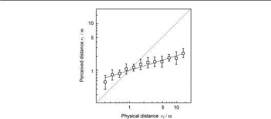
Although the ability of the human auditory system to estimate the sound source distance is generally poorer than the ability to locate sound source direction, a preliminary but biased auditory distance perception can still be formed. Experiments have demonstrated that the auditory system tends to significantly underestimate distances to distant sound sources with the physical source distance farther than a rough average of 1.6 m and typically overestimates distances to nearby sound sources with the physical source distance less than a rough average of 1.6 m. This finding suggests that the perceived source distance is not always identical to the physical one. Zahorik (2002a) examined experimental data from a variety of studies and found that the relationship between the perceived distance rI and the physical distance rS can be well approximated with a compressive power function by using a linear fit method:

Sound field, spatial hearing, and sound reproduction 45

Figure 1.24 Relationship between rI and rS obtained using a linear fit for a typical subject, with α = 0.32 and κ = 1.00 (Zahorik, 2002b, with the permission of Zahorik P.).

where κ is a constant whose average is slightly greater than 1 (average of approximately 1.32), and δ is a power-law exponent whose value is influenced by various factors, such as experimental conditions and subjects, so this value varies in a wide range with a rough average of 0.4. In the logarithmic coordinate, the relationship between rI and rS is expressed with straight lines having various slopes; among them, a straight line through the origin with a slope of 1 means that rI is identical to rS, i.e., the case of unbiased distance estimation. Figure 1.24 shows the relationship between rI and rS obtained using a linear fit for a typical subject (Zahorik, 2002b).

Auditory distance perception, which was thoroughly reviewed by Zahorik et al. (2005), is a complex and comprehensive process based on multiple cues. Subjective loudness has been considered an effective cue to distance perception. Generally, loudness is closely related to sound pressure or intensity at a listener’s position; usually, strong sound pressure results in high loudness. In a free field, the sound pressure generated by a point sound source with constant power is inversely proportional to the distance between the sound source and the receiver (the 1/r law); that is, the SPL decreases by 6 dB for each doubling of the source distance. As a result, a close distance corresponds to a high sound pressure and subsequent high loudness. As such, loudness becomes a cue for distance estimation. However, the 1/r law only applies to the free field and deviates in reflective environments. Moreover, the sound pressure and loudness at a listener’s position depends on source properties, such as radiated power. Previous knowledge on sound sources or stimuli also influences the performance of distance estimation when loudness-based cues are used. In general, loudness is regarded as a relative distance cue unless the listener is highly familiar with the pressure level of the sound source.

The high-frequency attenuation caused by air absorption may be another cue of auditory distance perception. For a far sound source, air absorption acts as a low-pass filter and thereby modifies the spectra of sound pressures at the receiving position. This effect is important only for an extremely far sound source and negligible in an ordinary-sized room. Moreover, previous knowledge on the sound source may influence the performance of distance estimation when high-frequency attenuation-based cues are used. In general, highfrequency attenuation provides weak information for relative distance perception.

Some studies have demonstrated that the effects of acoustic diffraction and shadowing by the head provide information on evaluating distance for nearby sound sources (Brungart and Rabinowitz, 1999; Brungart et al., 1999; Brungart, 1999). In Section 1.6.2, ILD is nearly