
- •Preface
- •Introduction
- •1.1 Spatial coordinate systems
- •1.2 Sound fields and their physical characteristics
- •1.2.1 Free-field and sound waves generated by simple sound sources
- •1.2.2 Reflections from boundaries
- •1.2.3 Directivity of sound source radiation
- •1.2.4 Statistical analysis of acoustics in an enclosed space
- •1.2.5 Principle of sound receivers
- •1.3 Auditory system and perception
- •1.3.1 Auditory system and its functions
- •1.3.2 Hearing threshold and loudness
- •1.3.3 Masking
- •1.3.4 Critical band and auditory filter
- •1.4 Artificial head models and binaural signals
- •1.4.1 Artificial head models
- •1.4.2 Binaural signals and head-related transfer functions
- •1.5 Outline of spatial hearing
- •1.6 Localization cues for a single sound source
- •1.6.1 Interaural time difference
- •1.6.2 Interaural level difference
- •1.6.3 Cone of confusion and head movement
- •1.6.4 Spectral cues
- •1.6.5 Discussion on directional localization cues
- •1.6.6 Auditory distance perception
- •1.7 Summing localization and spatial hearing with multiple sources
- •1.7.1 Summing localization with two sound sources
- •1.7.2 The precedence effect
- •1.7.3 Spatial auditory perceptions with partially correlated and uncorrelated source signals
- •1.7.4 Auditory scene analysis and spatial hearing
- •1.7.5 Cocktail party effect
- •1.8 Room reflections and auditory spatial impression
- •1.8.1 Auditory spatial impression
- •1.8.2 Sound field-related measures and auditory spatial impression
- •1.8.3 Binaural-related measures and auditory spatial impression
- •1.9.1 Basic principle of spatial sound
- •1.9.2 Classification of spatial sound
- •1.9.3 Developments and applications of spatial sound
- •1.10 Summary
- •2.1 Basic principle of a two-channel stereophonic sound
- •2.1.1 Interchannel level difference and summing localization equation
- •2.1.2 Effect of frequency
- •2.1.3 Effect of interchannel phase difference
- •2.1.4 Virtual source created by interchannel time difference
- •2.1.5 Limitation of two-channel stereophonic sound
- •2.2.1 XY microphone pair
- •2.2.2 MS transformation and the MS microphone pair
- •2.2.3 Spaced microphone technique
- •2.2.4 Near-coincident microphone technique
- •2.2.5 Spot microphone and pan-pot technique
- •2.2.6 Discussion on microphone and signal simulation techniques for two-channel stereophonic sound
- •2.3 Upmixing and downmixing between two-channel stereophonic and mono signals
- •2.4 Two-channel stereophonic reproduction
- •2.4.1 Standard loudspeaker configuration of two-channel stereophonic sound
- •2.4.2 Influence of front-back deviation of the head
- •2.5 Summary
- •3.1 Physical and psychoacoustic principles of multichannel surround sound
- •3.2 Summing localization in multichannel horizontal surround sound
- •3.2.1 Summing localization equations for multiple horizontal loudspeakers
- •3.2.2 Analysis of the velocity and energy localization vectors of the superposed sound field
- •3.2.3 Discussion on horizontal summing localization equations
- •3.3 Multiple loudspeakers with partly correlated and low-correlated signals
- •3.4 Summary
- •4.1 Discrete quadraphone
- •4.1.1 Outline of the quadraphone
- •4.1.2 Discrete quadraphone with pair-wise amplitude panning
- •4.1.3 Discrete quadraphone with the first-order sound field signal mixing
- •4.1.4 Some discussions on discrete quadraphones
- •4.2 Other horizontal surround sounds with regular loudspeaker configurations
- •4.2.1 Six-channel reproduction with pair-wise amplitude panning
- •4.2.2 The first-order sound field signal mixing and reproduction with M ≥ 3 loudspeakers
- •4.3 Transformation of horizontal sound field signals and Ambisonics
- •4.3.1 Transformation of the first-order horizontal sound field signals
- •4.3.2 The first-order horizontal Ambisonics
- •4.3.3 The higher-order horizontal Ambisonics
- •4.3.4 Discussion and implementation of the horizontal Ambisonics
- •4.4 Summary
- •5.1 Outline of surround sounds with accompanying picture and general uses
- •5.2 5.1-Channel surround sound and its signal mixing analysis
- •5.2.1 Outline of 5.1-channel surround sound
- •5.2.2 Pair-wise amplitude panning for 5.1-channel surround sound
- •5.2.3 Global Ambisonic-like signal mixing for 5.1-channel sound
- •5.2.4 Optimization of three frontal loudspeaker signals and local Ambisonic-like signal mixing
- •5.2.5 Time panning for 5.1-channel surround sound
- •5.3 Other multichannel horizontal surround sounds
- •5.4 Low-frequency effect channel
- •5.5 Summary
- •6.1 Summing localization in multichannel spatial surround sound
- •6.1.1 Summing localization equations for spatial multiple loudspeaker configurations
- •6.1.2 Velocity and energy localization vector analysis for multichannel spatial surround sound
- •6.1.3 Discussion on spatial summing localization equations
- •6.1.4 Relationship with the horizontal summing localization equations
- •6.2 Signal mixing methods for a pair of vertical loudspeakers in the median and sagittal plane
- •6.3 Vector base amplitude panning
- •6.4 Spatial Ambisonic signal mixing and reproduction
- •6.4.1 Principle of spatial Ambisonics
- •6.4.2 Some examples of the first-order spatial Ambisonics
- •6.4.4 Recreating a top virtual source with a horizontal loudspeaker arrangement and Ambisonic signal mixing
- •6.5 Advanced multichannel spatial surround sounds and problems
- •6.5.1 Some advanced multichannel spatial surround sound techniques and systems
- •6.5.2 Object-based spatial sound
- •6.5.3 Some problems related to multichannel spatial surround sound
- •6.6 Summary
- •7.1 Basic considerations on the microphone and signal simulation techniques for multichannel sounds
- •7.2 Microphone techniques for 5.1-channel sound recording
- •7.2.1 Outline of microphone techniques for 5.1-channel sound recording
- •7.2.2 Main microphone techniques for 5.1-channel sound recording
- •7.2.3 Microphone techniques for the recording of three frontal channels
- •7.2.4 Microphone techniques for ambience recording and combination with frontal localization information recording
- •7.2.5 Stereophonic plus center channel recording
- •7.3 Microphone techniques for other multichannel sounds
- •7.3.1 Microphone techniques for other discrete multichannel sounds
- •7.3.2 Microphone techniques for Ambisonic recording
- •7.4 Simulation of localization signals for multichannel sounds
- •7.4.1 Methods of the simulation of directional localization signals
- •7.4.2 Simulation of virtual source distance and extension
- •7.4.3 Simulation of a moving virtual source
- •7.5 Simulation of reflections for stereophonic and multichannel sounds
- •7.5.1 Delay algorithms and discrete reflection simulation
- •7.5.2 IIR filter algorithm of late reverberation
- •7.5.3 FIR, hybrid FIR, and recursive filter algorithms of late reverberation
- •7.5.4 Algorithms of audio signal decorrelation
- •7.5.5 Simulation of room reflections based on physical measurement and calculation
- •7.6 Directional audio coding and multichannel sound signal synthesis
- •7.7 Summary
- •8.1 Matrix surround sound
- •8.1.1 Matrix quadraphone
- •8.1.2 Dolby Surround system
- •8.1.3 Dolby Pro-Logic decoding technique
- •8.1.4 Some developments on matrix surround sound and logic decoding techniques
- •8.2 Downmixing of multichannel sound signals
- •8.3 Upmixing of multichannel sound signals
- •8.3.1 Some considerations in upmixing
- •8.3.2 Simple upmixing methods for front-channel signals
- •8.3.3 Simple methods for Ambient component separation
- •8.3.4 Model and statistical characteristics of two-channel stereophonic signals
- •8.3.5 A scale-signal-based algorithm for upmixing
- •8.3.6 Upmixing algorithm based on principal component analysis
- •8.3.7 Algorithm based on the least mean square error for upmixing
- •8.3.8 Adaptive normalized algorithm based on the least mean square for upmixing
- •8.3.9 Some advanced upmixing algorithms
- •8.4 Summary
- •9.1 Each order approximation of ideal reproduction and Ambisonics
- •9.1.1 Each order approximation of ideal horizontal reproduction
- •9.1.2 Each order approximation of ideal three-dimensional reproduction
- •9.2 General formulation of multichannel sound field reconstruction
- •9.2.1 General formulation of multichannel sound field reconstruction in the spatial domain
- •9.2.2 Formulation of spatial-spectral domain analysis of circular secondary source array
- •9.2.3 Formulation of spatial-spectral domain analysis for a secondary source array on spherical surface
- •9.3 Spatial-spectral domain analysis and driving signals of Ambisonics
- •9.3.1 Reconstructed sound field of horizontal Ambisonics
- •9.3.2 Reconstructed sound field of spatial Ambisonics
- •9.3.3 Mixed-order Ambisonics
- •9.3.4 Near-field compensated higher-order Ambisonics
- •9.3.5 Ambisonic encoding of complex source information
- •9.3.6 Some special applications of spatial-spectral domain analysis of Ambisonics
- •9.4 Some problems related to Ambisonics
- •9.4.1 Secondary source array and stability of Ambisonics
- •9.4.2 Spatial transformation of Ambisonic sound field
- •9.5 Error analysis of Ambisonic-reconstructed sound field
- •9.5.1 Integral error of Ambisonic-reconstructed wavefront
- •9.5.2 Discrete secondary source array and spatial-spectral aliasing error in Ambisonics
- •9.6 Multichannel reconstructed sound field analysis in the spatial domain
- •9.6.1 Basic method for analysis in the spatial domain
- •9.6.2 Minimizing error in reconstructed sound field and summing localization equation
- •9.6.3 Multiple receiver position matching method and its relation to the mode-matching method
- •9.7 Listening room reflection compensation in multichannel sound reproduction
- •9.8 Microphone array for multichannel sound field signal recording
- •9.8.1 Circular microphone array for horizontal Ambisonic recording
- •9.8.2 Spherical microphone array for spatial Ambisonic recording
- •9.8.3 Discussion on microphone array recording
- •9.9 Summary
- •10.1 Basic principle and implementation of wave field synthesis
- •10.1.1 Kirchhoff–Helmholtz boundary integral and WFS
- •10.1.2 Simplification of the types of secondary sources
- •10.1.3 WFS in a horizontal plane with a linear array of secondary sources
- •10.1.4 Finite secondary source array and effect of spatial truncation
- •10.1.5 Discrete secondary source array and spatial aliasing
- •10.1.6 Some issues and related problems on WFS implementation
- •10.2 General theory of WFS
- •10.2.1 Green’s function of Helmholtz equation
- •10.2.2 General theory of three-dimensional WFS
- •10.2.3 General theory of two-dimensional WFS
- •10.2.4 Focused source in WFS
- •10.3 Analysis of WFS in the spatial-spectral domain
- •10.3.1 General formulation and analysis of WFS in the spatial-spectral domain
- •10.3.2 Analysis of the spatial aliasing in WFS
- •10.3.3 Spatial-spectral division method of WFS
- •10.4 Further discussion on sound field reconstruction
- •10.4.1 Comparison among various methods of sound field reconstruction
- •10.4.2 Further analysis of the relationship between acoustical holography and sound field reconstruction
- •10.4.3 Further analysis of the relationship between acoustical holography and Ambisonics
- •10.4.4 Comparison between WFS and Ambisonics
- •10.5 Equalization of WFS under nonideal conditions
- •10.6 Summary
- •11.1 Basic principles of binaural reproduction and virtual auditory display
- •11.1.1 Binaural recording and reproduction
- •11.1.2 Virtual auditory display
- •11.2 Acquisition of HRTFs
- •11.2.1 HRTF measurement
- •11.2.2 HRTF calculation
- •11.2.3 HRTF customization
- •11.3 Basic physical features of HRTFs
- •11.3.1 Time-domain features of far-field HRIRs
- •11.3.2 Frequency domain features of far-field HRTFs
- •11.3.3 Features of near-field HRTFs
- •11.4 HRTF-based filters for binaural synthesis
- •11.5 Spatial interpolation and decomposition of HRTFs
- •11.5.1 Directional interpolation of HRTFs
- •11.5.2 Spatial basis function decomposition and spatial sampling theorem of HRTFs
- •11.5.3 HRTF spatial interpolation and signal mixing for multichannel sound
- •11.5.4 Spectral shape basis function decomposition of HRTFs
- •11.6 Simplification of signal processing for binaural synthesis
- •11.6.1 Virtual loudspeaker-based algorithms
- •11.6.2 Basis function decomposition-based algorithms
- •11.7.1 Principle of headphone equalization
- •11.7.2 Some problems with binaural reproduction and VAD
- •11.8 Binaural reproduction through loudspeakers
- •11.8.1 Basic principle of binaural reproduction through loudspeakers
- •11.8.2 Virtual source distribution in two-front loudspeaker reproduction
- •11.8.3 Head movement and stability of virtual sources in Transaural reproduction
- •11.8.4 Timbre coloration and equalization in transaural reproduction
- •11.9 Virtual reproduction of stereophonic and multichannel surround sound
- •11.9.1 Binaural reproduction of stereophonic and multichannel sound through headphones
- •11.9.2 Stereophonic expansion and enhancement
- •11.9.3 Virtual reproduction of multichannel sound through loudspeakers
- •11.10.1 Binaural room modeling
- •11.10.2 Dynamic virtual auditory environments system
- •11.11 Summary
- •12.1 Physical analysis of binaural pressures in summing virtual source and auditory events
- •12.1.1 Evaluation of binaural pressures and localization cues
- •12.1.2 Method for summing localization analysis
- •12.1.3 Binaural pressure analysis of stereophonic and multichannel sound with amplitude panning
- •12.1.4 Analysis of summing localization with interchannel time difference
- •12.1.5 Analysis of summing localization at the off-central listening position
- •12.1.6 Analysis of interchannel correlation and spatial auditory sensations
- •12.2 Binaural auditory models and analysis of spatial sound reproduction
- •12.2.1 Analysis of lateral localization by using auditory models
- •12.2.2 Analysis of front-back and vertical localization by using a binaural auditory model
- •12.2.3 Binaural loudness models and analysis of the timbre of spatial sound reproduction
- •12.3 Binaural measurement system for assessing spatial sound reproduction
- •12.4 Summary
- •13.1 Analog audio storage and transmission
- •13.1.1 45°/45° Disk recording system
- •13.1.2 Analog magnetic tape audio recorder
- •13.1.3 Analog stereo broadcasting
- •13.2 Basic concepts of digital audio storage and transmission
- •13.3 Quantization noise and shaping
- •13.3.1 Signal-to-quantization noise ratio
- •13.3.2 Quantization noise shaping and 1-Bit DSD coding
- •13.4 Basic principle of digital audio compression and coding
- •13.4.1 Outline of digital audio compression and coding
- •13.4.2 Adaptive differential pulse-code modulation
- •13.4.3 Perceptual audio coding in the time-frequency domain
- •13.4.4 Vector quantization
- •13.4.5 Spatial audio coding
- •13.4.6 Spectral band replication
- •13.4.7 Entropy coding
- •13.4.8 Object-based audio coding
- •13.5 MPEG series of audio coding techniques and standards
- •13.5.1 MPEG-1 audio coding technique
- •13.5.2 MPEG-2 BC audio coding
- •13.5.3 MPEG-2 advanced audio coding
- •13.5.4 MPEG-4 audio coding
- •13.5.5 MPEG parametric coding of multichannel sound and unified speech and audio coding
- •13.5.6 MPEG-H 3D audio
- •13.6 Dolby series of coding techniques
- •13.6.1 Dolby digital coding technique
- •13.6.2 Some advanced Dolby coding techniques
- •13.7 DTS series of coding technique
- •13.8 MLP lossless coding technique
- •13.9 ATRAC technique
- •13.10 Audio video coding standard
- •13.11 Optical disks for audio storage
- •13.11.1 Structure, principle, and classification of optical disks
- •13.11.2 CD family and its audio formats
- •13.11.3 DVD family and its audio formats
- •13.11.4 SACD and its audio formats
- •13.11.5 BD and its audio formats
- •13.12 Digital radio and television broadcasting
- •13.12.1 Outline of digital radio and television broadcasting
- •13.12.2 Eureka-147 digital audio broadcasting
- •13.12.3 Digital radio mondiale
- •13.12.4 In-band on-channel digital audio broadcasting
- •13.12.5 Audio for digital television
- •13.13 Audio storage and transmission by personal computer
- •13.14 Summary
- •14.1 Outline of acoustic conditions and requirements for spatial sound intended for domestic reproduction
- •14.2 Acoustic consideration and design of listening rooms
- •14.3 Arrangement and characteristics of loudspeakers
- •14.3.1 Arrangement of the main loudspeakers in listening rooms
- •14.3.2 Characteristics of the main loudspeakers
- •14.3.3 Bass management and arrangement of subwoofers
- •14.4 Signal and listening level alignment
- •14.5 Standards and guidance for conditions of spatial sound reproduction
- •14.6 Headphones and binaural monitors of spatial sound reproduction
- •14.7 Acoustic conditions for cinema sound reproduction and monitoring
- •14.8 Summary
- •15.1 Outline of psychoacoustic and subjective assessment experiments
- •15.2 Contents and attributes for spatial sound assessment
- •15.3 Auditory comparison and discrimination experiment
- •15.3.1 Paradigms of auditory comparison and discrimination experiment
- •15.3.2 Examples of auditory comparison and discrimination experiment
- •15.4 Subjective assessment of small impairments in spatial sound systems
- •15.5 Subjective assessment of a spatial sound system with intermediate quality
- •15.6 Virtual source localization experiment
- •15.6.1 Basic methods for virtual source localization experiments
- •15.6.2 Preliminary analysis of the results of virtual source localization experiments
- •15.6.3 Some results of virtual source localization experiments
- •15.7 Summary
- •16.1.1 Application to commercial cinema and related problems
- •16.1.2 Applications to domestic reproduction and related problems
- •16.1.3 Applications to automobile audio
- •16.2.1 Applications to virtual reality
- •16.2.2 Applications to communication and information systems
- •16.2.3 Applications to multimedia
- •16.2.4 Applications to mobile and handheld devices
- •16.3 Applications to the scientific experiments of spatial hearing and psychoacoustics
- •16.4 Applications to sound field auralization
- •16.4.1 Auralization in room acoustics
- •16.4.2 Other applications of auralization technique
- •16.5 Applications to clinical medicine
- •16.6 Summary
- •References
- •Index

38 Spatial Sound
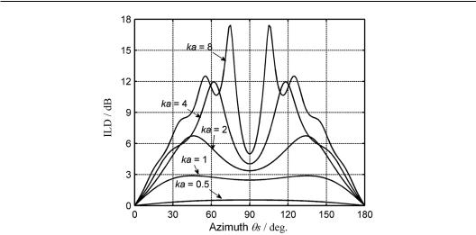
Figure 1.20 Calculated ILD as a function of azimuth at different ka with the spherical head model.
ILD varies dramatically with azimuth at high frequencies, such as ka of 4.0 and 8.0 (in Figure 1.20). Additionally, the maximum ILD for a sinusoidal sound stimulus (with a single frequency component) does not appear at an azimuth of 90°, where the contralateral ear is exactly opposite the sound source. This finding is due to the enhancement in sound pressure in the contralateral ear by the in-phase interference of multipath diffracted sounds around the spherical head. For a complex sound wave with multiple frequency components, such as octave noise, ILD varies relatively smoothly with azimuth. However, an actual human head is not a perfect sphere, and it is composed of the pinnae and other fine structures. Therefore, the relationship between ILD, sound source direction, and frequency is more complicated than that for a spherical head. Nevertheless, the results from the spherical head model are adequate for qualitatively interpreting some localization phenomena.
1.6.3 Cone of confusion and head movement
ITD and ILD are regarded as two dominant localization cues at low and high frequencies, respectively, which were first stated in classic “duplex theory” proposed by Lord Rayleigh in 1907. However, a set of ITD and ILD are inadequate for determining the unique position of a sound source. In fact, an infinite number of spatial positions possess identical differences in path lengths to the two ears (i.e., identical ITD). When the curved surface of the spherical head is disregarded and when the two ears are approximated by two separated points in a free space, the points with identical ITD form a cone around the interaural axis in a threedimensional space, which is called “cone of confusion” (Figure 1.21). In the cone of confusion, ITD alone is insufficient for determining an exclusive sound source position. Similarly, for a spherical head model and at a far-field distance comparatively longer than the head radius, an infinite point set exists in space within which the ILDs are identical for all points. For an actual human head, even when its nonspherical form and curved surface are considered, the corresponding ITD and ILD are still insufficient for identifying the unique position of a sound source because they do not vary monotonously with the source position. In this case, the cone of confusion persists, but it is no longer a strict cone.
An extreme case of the cone of confusion is the median plane in which the sound pressures received by the two ears are nearly identical; thus, ITD and ILD are zero. In another case, two sound sources are located at the front–back mirror positions at the azimuths of 45° and

Sound field, spatial hearing, and sound reproduction 39
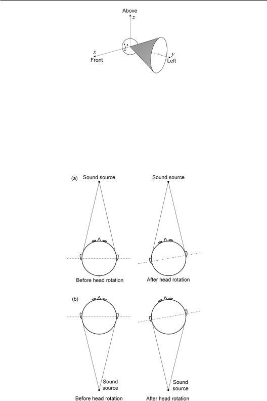
Figure 1.21 Cone of confusion in sound source localization.
135° in the horizontal plane. The resultant ITD and ILD for the two sound source positions are identical as far as a symmetrical spherical head is concerned. ITD and ILD can determine only the cone of confusion in which the sound source is located but not the unique spatial position of the sound source. Therefore, Rayleigh’s duplex theory is only effective for lateral localization and ineffective for the front–back and vertical localization.
To address this problem, Wallach (1940) hypothesized that ITD and ILD change introduced by head-turning may be another localization cue (i.e., a dynamic cue). For example, when the head in Figure 1.22 is fixed, ITDs and ILDs for sources at the front (0°) and rear (180°) in the
Figure 1.22 Changes in ITD caused by head rotation: sound sources in the (a) front and (b) the rear.

40 Spatial Sound
horizontal plane are both zero because of the symmetry of the head. Hence, the two source positions are indistinguishable in terms of ITD and ILD cues. However, head rotation can introduce a change in ITD. If the head is rotated anticlockwise (to the left) around the vertical axis, the right ear comes closer to the front sound source, and the left ear comes closer to the rear sound source. That is, for the same head rotation, the ITD for the front sound source changes from zero to negative; by contrast, the ITD for the rear sound source changes from zero to positive. If the head is rotated clockwise (to the right) around the vertical axis, a completely opposite situation occurs. Head rotation changes not only the ITD but also the ILD and the sound pressure spectra in the ears, although ILD is not a monotonic function of the source azimuth. Therefore, dynamic information aids localization. Previous experiments preliminarily confirmed that head rotation around a vertical axis is necessary to resolve the front–back ambiguity in horizontal localization. This conclusion has been further verified by some recent experiments (Wightman and Kistler, 1999) and applied to virtual auditory displays (Section 11.10.2). In addition, experimental evidence has indicated that the change in ITD provides major dynamic information about front–back localization (Macpherson, 2011).
Wallach also hypothesized that head-turning provides information for vertical localization. Follow-up studies have attempted to verify this hypothesis through experiments. However, completely and experimentally excluding contributions from other vertical localization cues (such as spectral cues; Section 1.6.4) was difficult. Wallach’s hypothesis was not widely explored because of the lack of sufficient experimental support. Since the 1990s, nevertheless, the problem of vertical localization has attracted renewed attention to develop a virtual auditory display. Perrett and Noble (1997) first experimentally verified Wallach’s hypothesis. Our own work (Rao and Xie, 2005) further demonstrated that the change in ITD introduced by the head movement in two degrees of freedom (turning around the vertical and front–back axes, respectively, i.e., rotating and pivoting or yawing and rolling) provides information for localization in the median plane at low frequencies and allows the quantitative verification of Wallach’s hypothesis to be given (Chapter 6). Some recent experiments have also confirmed the contributions of head-turning to vertical localization (Ashby et al., 2013, 2014). In addition, other experiments have investigated the range and pattern of head movement made by listeners (Kim et al., 2013).
1.6.4 Spectral cues
Many studies have suggested that the spectral feature caused by the reflection and diffraction in the pinna and around the head and torso provides helpful information on vertical localization and front-back disambiguity. In contrast to binaural cues (ITD and ILD), the spectral cue is a monaural cue (Wightman and Kistler, 1997).
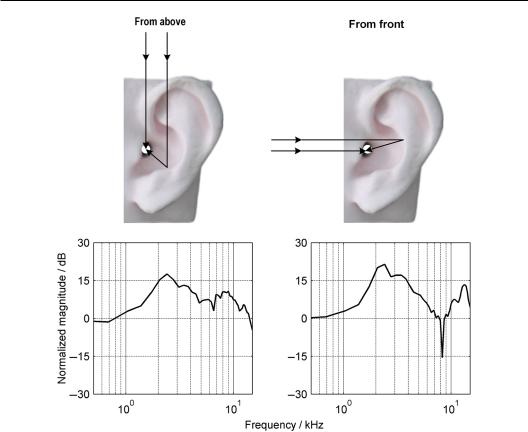
Batteau (1967) proposed a simplified model to explain the pinna effect. Figure 1.23 shows that direct and reflected sounds arrive at the entrance to the ear canal. The relative delay between the direct and reflected sounds is direction dependent because the incident sounds from different spatial directions are likely to be reflected by the different parts of the pinna. Therefore, peaks and notches in the sound pressure spectra caused by the interference between the direct and reflected sounds are also direction dependent, thereby providing information for directional localization. In Batteau’s model, the pinna effect is described as a combination of two reflections with different magnitudes, i.e., A1 and A2, and different time delays, i.e., τ1 and τ2. Hence, the transfer function of the pinna, including one direct and two reflected sounds, is expressed as
H f 1 A1 exp j2 f 1 A2 exp j2 f 2 . |
(1.6.8) |

Sound field, spatial hearing, and sound reproduction 41
Figure 1.23 Pinna interacting with incident sounds from two typical directions.
Batteau’s model achieved limited success because of its considerable simplification. The dimension of the pinna is about 65 mm, so it functions effectively only if the frequency is above 2–3 kHz. At this frequency, the sound wavelength is comparable with the dimension of the pinna. Moreover, the effect of the pinna is prominent at frequencies above 5–6 kHz. The pinna also has a complex and irregular surface, so it cannot be regarded as a reflective plane from the perspective of geometrical acoustics within the entire audible frequency range. This characteristic is the inherent drawback of Batteau’s model. Further studies have pointed out that the pinna reflects and diffracts the incident sound in a complex manner (Lopez-Poveda and Meddis, 1996). The interference among direct and multipath reflected/diffracted sounds acts as a filter and then modifies the incident sound spectrum as direction-dependent notches and peaks. In addition, this interference is highly sensitive to the shape and dimension of the pinna, which differs among individuals. Therefore, the spectral information provided by the pinna is an extremely individualized localization cue.
Shaw and Teranishi (1968) and Shaw (1974) investigated the effect of the pinna in terms of wave acoustics and proposed a resonance model, which demonstrates that resonances within pinna cavities and the ear canal form a series of resonance modes at mid and high frequencies of 3, 5, 9, 11, and 13 kHz. This model successfully interprets the peaks in the pressure spectra; among them, the peak at 3 kHz for the first salient resonance is derived from the quarter wavelength resonance of the ear canal, though the existence of the pinna extends the effective length of the ear canal. Hearing is also most sensitive around this frequency (Section 1.3.2). Moreover, the magnitudes of high-order resonance modes vary with the direction of