

24 |
2 Mechanic and Acoustic Oscillations |
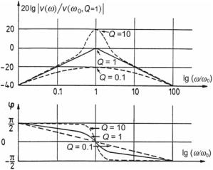
Fig. 2.6 Double-logarithmic plot of resonance curves of the velocity, illustrating the influence of the sharpness-of-resonance factor, Q
2.5 Energies and Dissipation Losses
To derive the energies and losses in the elements from which the oscillator is built, (2.13) is first multiplied with v(t ) to arrive at what is called instantaneous power, namely
|
dv |
|
1 |
|
|
dξ |
|
|||
P (t ) = F (t ) v(t ) = m |
v(t ) + r v2 |
|
|
|
|
|
|
|||
|
|
|
|
|
|
|||||
|
(t ) + |
|
v(t ) v(t ) dt . |
(2.33) |
||||||
dt |
n |
|||||||||
Integration over time then leads to a term with the dimension energy (work) as follows,
|
t1 |
dξ |
t1 |
dv |
|
t1 |
1 |
|
t1 |
||
|
|
|
|
||||||||
W 0, t1 = |
|
F (t ) v dt = m |
|
v |
|
dt + r |
|
v2dt + |
|
|
ξ v dt . (2.34) |
0 |
0 |
dt |
0 |
n |
0 |
||||||
For the case that the motion of the oscillator starts from its resting position, that is, for ξ t =0 = 0, this expression mutates to
ξ1 |
|
1 |
|
|
t1 |
1 |
1 |
|
|
||
|
F (t ) dξ = |
|
|
m v12 + r |
|
v2dt + |
|
|
|
ξ12 . |
(2.35) |
0 |
2 |
0 |
2 |
n |
|||||||
The left term denotes the energy that is fed into the system. The terms on the right side of the equality sign stand, from left to right, for the kinetic energy of the mass, the frictional losses (dissipation) in the dashpot, and the potential energy in the spring.
Our discussion starts with the case of no losses, that is, when r ≡ 0. In this case, the total energy in the system does not change. It simply swings between the mass
2.5 Energies and Dissipation Losses |
|
|
|
|
|
25 |
and the spring. We express these relationships as follows, |
|
|||||
W = |
1 |
m v2(t ) + |
1 |
ξ2(t ) . |
(2.36) |
|
|
|
|
||||
2 |
2n |
|||||
At the instant ξ = 0, all energy is kinetic, and when we have v = 0, all energy is potential. In mathematical terms, this is
|
ξ = |
|
= |
2 |
ˆ |
= |
|
= |
|
= 2n |
ˆ |
|
|
|
W ( |
|
0) |
|
|
1 |
m v2 |
|
W (v |
|
0) |
1 |
ξ |
2 . |
(2.37) |
|
|
|
|
|
|
|
||||||||
When losses are present due to friction, that is, when r = 0, the stationary state is maintained by a driving force. Recall that this section discusses force-driven oscillation. To keep the oscillation amplitude constant, the system requires supplementary power. This power results from the middle term of (2.35) and amounts to
|
|
t1 |
|
d |
|
t1 |
|
Wr = r |
|
v2(t )dt , |
and, thus Pr = r |
|
|
v2(t )dt . |
(2.38) |
0 |
dt |
0 |
Averaging over a full period, T , with the arbitrary phase, φ, we find
|
|
1 |
T |
vˆ2 cos2(ωt + φ)dt |
|
|
|
|
|
|
|||||||
P = r |
|
|
|
|
|
|
|
|
|||||||||
T |
0 |
|
|
|
|
|
|
||||||||||
= |
1 |
r v2 |
T |
= |
1 |
r v2 |
= |
1 |
F v |
F |
|
v |
|
. |
(2.39) |
||
|
|
|
|
|
|
||||||||||||
2 T |
2 |
2 |
|
|
|||||||||||||
ˆ |
|
ˆ |
ˆ ˆ = |
|
rms |
|
rms |
|
|
||||||||
At the dashpot, v and F are in phase, which means that the supplied power is purely resistive (active) power. This holds for the complete system when driven at its characteristic frequency. Off this frequency, additional (reactive) power is needed to keep the system stationarily oscillating.
2.6 Basic Elements of Linear, Oscillating, Acoustic Systems
In addition to the mechanic elements, there is a further class of elements for oscillators that are traditionally called acoustic elements. Note that the terms mechanic and acoustic are historic in this case. Since sound is mechanic, the oscillators built from both classes of elements are, to be sure, mechanic and acoustic at the same time.
The acoustic elements are formed by small cavities filled with fluid, that is, gas or liquid. To deal with these cavities as concentrated elements, their linear dimensions must be small compared to the wavelengths under consideration. To define the acoustic elements, this section uses the sound pressure, p, the sound-pressure difference, p = p1 − p2, and the volume velocity,
q = |
dV |
= A |
dξ |
= A v(t ) . |
(2.40) |
dt |
dt |
26 |
2 Mechanic and Acoustic Oscillations |
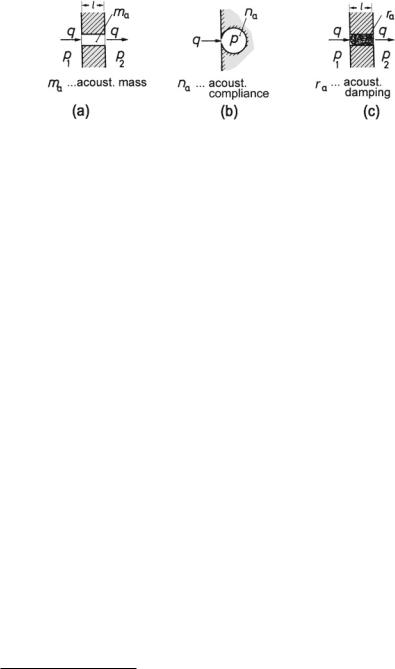
Fig. 2.7 Basic elements of linear acoustic oscillators. (a) Acoustic mass. (b) Acoustic spring.
(c) Acoustic damper
Figure 2.7 schematically illustrates the three acoustic elements—acoustic mass, ma , acoustic spring, na , and acoustic damper, ra . Note that here the damper and the mass are two-port elements while the spring has only one port.
The following equations define these elements.
• Acoustic Mass |
|
|
|
|
|
|
|
|
|
|
|
|
|
|
|
|
|
|||
p (t ) = ma |
dq |
or, in complex notation, |
p |
= j ω ma |
q |
|
|
(2.41) |
||||||||||||
|
|
|
|
|||||||||||||||||
dt |
||||||||||||||||||||
|
|
|
|
|||||||||||||||||
• Acoustic Spring |
|
|
|
|
|
|
|
|
|
|
|
|
|
|
|
|
|
|||
1 |
|
|
|
|
|
|
|
1 |
|
|
|
|
|
|
||||||
p(t ) = |
|
|
q dt |
|
or, in complex notation, |
p |
= |
|
|
|
q |
(2.42) |
||||||||
na |
|
j ω na |
||||||||||||||||||
|
|
|
|
|
|
|
|
|
|
|
|
|
||||||||
• Acoustic Damper5 |
|
|
|
|
|
|
|
|
|
|
|
|
|
|
|
|
|
|||
p (t ) = ra q |
or, in complex notation, |
|
|
p |
= ra |
q |
|
(2.43) |
||||||||||||
|
|
|
|
|
|
|
|
|||||||||||||
2.7 The Helmholtz Resonator
The Helmholtz resonator is the best-known example of an oscillator with an acoustic element. A Helmholtz resonator is commonly demonstrated by blowing over the open end of a bottle to produce a musical tone. This is an auditory event with a distinct pitch, which is adjustable by filling the bottle with some water.
5 For the characteristic parameters of the acoustic elements, the following relations hold: ma =− l/ A with − being density, na = V /(η p− ) = V /c2 − with V being volume, η = cp/cv, and ra = Ξ l/ A with Ξ being flow resistivity—for details refer to Sect. 11.5.
2.7 The Helmholtz Resonator |
27 |
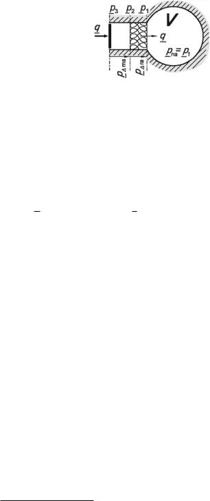
Fig. 2.8 Helmholtz resonator with friction
What happens when the bottle is blown on? The air in the bottleneck is a mass oscillating on the air inside the bottle, and the air inside the bottle acts as a spring.6 Figure 2.8 schematically illustrates the Helmholtz resonator with friction that causes damping. The three elements, mass, damping, and spring, are connected in
cascade (chain), so that the total pressure results in
p |
= |
p |
ma + |
p |
ra + |
p |
na . |
(2.44) |
|
|
|
|
|
Dividing p by the volume velocity, q, delivers the acoustic impedance, Z a , namely,
|
p |
1 |
|
|
||||
Z a = |
|
|
|
= j ω ma + ra + |
|
. |
(2.45) |
|
|
|
|
||||||
|
q |
|
j ω na |
|||||
2.8 Exercises
Differential Equations, Free and Forced Oscillation, Resonance Curves, Complex Power in Mechanic Systems
Problem 2.1
(a)Given a (constant) mass, m, describe/sketch the mechanic impedance of the mass as a function of the angular frequency, ω. Determine the phase angle of its mechanic impedance.
(b)Given a (constant) compliance, n, describe/sketch the mechanic impedance of the spring as a function of the angular frequency, ω. Determine the phase angle of its mechanic impedance.
Problem 2.2 Given a mechanic parallel oscillator with mass, m, compliance, n, and damping, r .
(a) Establish a corresponding differential equation for a harmonic force exci-
F cos |
ω |
t , expressed in a suitable quantity. |
tation, F0 = ˆ0 |
|
6 Usually the spring characteristics of air are not directly experienced because the air evacuates. Yet, in this case, the effect is similar to operating a tire pump with the opening hole pressed closed.
28 |
2 Mechanic and Acoustic Oscillations |
(b)Find a solution to the differential equation if there is no external excitation.
(c)Find the possible types of solutions of the differential equation for excitation as given in (a).
Problem 2.3 A mechanic parallel oscillator be excited by a sinusoidal force of constant amplitude, F0 = const , which is independent of frequency.
(a)Calculate and plot the trajectory of the velocity, v, in the complex plane as a function of frequency, f .
(b)Find the relationship between the damping coefficient, δ = r/2 m, and the bandwidth, ω , as defined by the half-value (−3 dB) on the resonance curve.
(c)Quantitatively explain the following statement, which is applicable for the determination of the sharpness-of-resonance factor, Q, by inspection of an oscilloscopic plot.
“The quality factor” approximately represents the number of oscillations of a damped oscillation that precede a 96%-reduction of the starting amplitude.
Problem 2.4 A parallel mechanic oscillator contains a mass, m = 0.63 Ns2/m, a spring with a compliance of, n = 0.027 m/N, and a damper with r = 6.02 Ns/m.
Determine for this parallel mechanic oscillator
–The resonance frequency, f0
–The damping coefficient, δ
–The sharpness-of-resonance factor, Q and the decay time, Td
–Will this system be oscillating or not?
Problem 2.5 Discuss why the complex power in a mechanic-oscillator system is
P |
= |
1 |
F v . |
(2.46) |
|
2 |
|||||
|
|
|
Problem 2.6 Given a lossy electric series resonator as shown in Fig. 1.3.
(a)Determine the following quantities using a graph in the complex plane: input impedance Z , input admittance Y , resonance frequency ω0, characteristic resistance Z 0.
(b)Derive the relation between bandwidth, ω , and sharpness-of-resonance factor, Q.
2.8 Exercises |
29 |
(c)Plot the magnitude of the input impedance, Y , as a function of the angular frequency in double-logarithmic representation.
Problem 2.7 For a parallel mechanic oscillator, show that the phase of ξ, concerning the excitation, becomes − π2 at the characteristic frequency of the forced oscillation, ω0, when a sinusoidal excitation with constant amplitude is applied.

Chapter 3
Electromechanic and Electroacoustic
Analogies
During our discussion of the simple mechanic and acoustic oscillators in Chap. 2, readers with some electrical engineering experience may have realized that many mathematical formulas are similar to those that appear when dealing with electric oscillators. There is a general isomorphism of the equations in mechanic, acoustic, and electric networks. This allows to describe mechanic and acoustic networks via analog electric ones. Formulation in electrical-coordinates is often to the advantage of those who are familiar with the theory of electric networks since analysis and synthesis methods from network theory are easily and figuratively applied.
There is more than one way to portray a mechanic or acoustic network by an analog electric one, depending on the coordinates used. There is never the best analogy but rather one which is optimal for the specific application considered. Also, note that analogies have limits of validity. If they mimicked the problem completely, they would cease to be analogies.
For electrical engineers, dealing with mechanic and acoustic networks in terms of their electric analogies means transforming uncommon problems into common ones, which is why they often prefer this method. Nevertheless, it is always possible to deal with the problems in their original form as well.
The following fundamental relations are to be considered when selecting coordinates for analog representations. The two terminals of an electric circuit serve to feed electric energy into the system or extracted it from it. In both cases, the two terminals form a port. By restricting ourselves to monofrequent (sinusoidal) signals, it is sufficient to consider complex power instead of energy.
Electric power is the complex product of the electric voltage, u, and the electric current, i—as derived in Sect. 16.2. Note that u and i denote electric coordinates in complex notation, with peak values as magnitudes. Thus, the complex electric power
is |
= |
1 |
u i , |
(3.1) |
P el |
|
|||
2 |
© Springer-Verlag GmbH Germany, part of Springer Nature 2021 |
31 |
N. Xiang and J. Blauert, Acoustics for Engineers, https://doi.org/10.1007/978-3-662-63342-7_3