

2.3 Free Oscillations of Parallel Mechanic Oscillators |
19 |
2.3 Free Oscillations of Parallel Mechanic Oscillators
This section deals with the particular case that the oscillator is in a position away from its resting position, and the introduced force is set to zero, that is, F (t ) = 0 for t > 0. The differential equation (2.13) then converts into a homogenous differential equation as follows,
d2ξ |
|
dξ |
1 |
|
|
||
m |
|
+ r |
|
+ |
|
ξ = 0 . |
(2.14) |
dt 2 |
dt |
n |
|||||
The solution of this equation is called free oscillation or eigen-oscillation of the system. A trial using ξ = e st results in the characteristic equation3
m s2 |
1 |
= 0 , |
|
+ r s + n |
(2.15) |
where s denotes the complex frequency. The general solution of this quadratic equation reads as
|
r |
|
r 2 |
1 |
|
|
|
|
|
± |
or s 1, 2 = −δ ± δ2 − ω02 , (2.16) |
||||||
s 1, 2 = − |
|
|
− |
|
||||
2 m |
4 m2 |
m n |
||||||
√
where δ = r/2m is the damping coefficient and ω0 = 1/ m n the characteristic angular frequency. This general form renders the three different types of solutions, namely,
Case (a) with δ = ω0 ... critical damping, only one root, which is real. Case (b) with δ > ω0 ... strong damping, both roots real, s is negative. Case (c) with δ < ω0 ... weak damping, both roots are complex.
The differential equation for a simple oscillator is of second order, making it necessary to have two initial conditions to derive specific solutions. Three forms of general solutions exist, which are listed below. It remains to adjust them to the particular initial conditions to finally arrive at particular solutions.
• Case (a) (δ = ω0)
ξ |
(t ) = ( |
ξ |
1 + |
ξ |
2) e−δt . |
(2.17) |
|
|
|
|
This case is at the brink of both periodic and aperiodic decay. Depending on the initial conditions, it may or may not render a single swing-over. It is called the aperiodic limiting case.
• Case (b) (δ > ω0) |
|
ξ(t ) = ξ 1 e−(δ−√δ2 −ω02 )t + ξ 2 e−(δ+√δ2 −ω02 )t . |
(2.18) |
3 As noted in the introduction to this chapter, the general exponential function is an eigen-function of linear differential equations. This means that it stays to be an exponential function when differentiated or integrated.
20 |
|
|
|
|
|
|
2 Mechanic and Acoustic Oscillations |
|||
This solution, called the creeping case, describes an aperiodic decay. |
|
|||||||||
• Case (c) (δ < ω0) |
|
|
|
|
||||||
|
ξ |
(t ) = |
ξ |
1 e−δt e−jωt + |
ξ |
2 e−δt e+jωt , |
with ω = ω02 − δ2 . |
(2.19) |
||
|
|
|
|
|
||||||
This solution, called the oscillating case, describes a periodic, decaying oscillation. It represents indeed an oscillation as illustrated by looking at the particular special case of ξ 1 = ξ 2 = ξ 1, 2/2.
Substituting it into (2.19) yields |
|
ξ(t ) = ξ 1, 2 e−δt cos(ωt ) |
(2.20) |
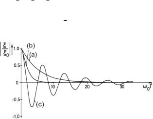
Fig. 2.3 Decays of a simple oscillator for different damping settings (schematic). (a) Aperiodic limiting case. (b) Aperiodic case. (c) Oscillating case
Figure 2.3 illustrates the three cases. The fastest-possible decay below a threshold— which, by the way, is the objective when tuning the suspension of road vehicles—is achieved with a slightly subcritical damping of δ ≈ 0.6 ω0.
In addition to δ = r/2m, the following two quantities are often used in acoustics to characterize the amount of damping in an oscillating system,
Q… The sharpness-of-resonance factor, also known as quality factor.
Td … The decay time—similar to the reverberation time in Sect. 12.5.
The sharpness-of-resonance factor, Q, is defined as |
|
||||
Q = |
ω0 |
= |
ω0 m |
, |
(2.21) |
2 δ |
r |
||||
It is a measure of the width of the peak of the resonance curve—compare Fig. 2.6. A more illustrative interpretation is possible in the time domain when one considers that after Q oscillations a mildly damped oscillation has decreased to 4 % of its starting value—which is at the brink of what is visually detectable on an oscilloscope
screen.

2.3 Free Oscillations of Parallel Mechanic Oscillators |
21 |
|
Table 2.1 Typical Q values for various oscillators |
|
|
|
|
|
Type of element |
Quality factor |
|
|
|
|
Electric oscillator of traditional construction |
Q ≈ 102–103 |
|
(coil, capacitor, resistor) |
|
|
Electromagnetic cavity oscillator |
Q ≈ 103–106 |
|
Mechanic oscillator, steel in vacuum |
Q ≈ 5 · 103 |
|
Quartz oscillator in vacuum |
Q ≈ 5 · 105 |
|
The decay time, Td, measures how long it takes for an oscillation to decrease by 60 dB after the excitation has been stopped. At this level, the velocity and displacement have decayed to one-thousandth and the power to one-millionth of its original value. Td and δ are related by Td ≈ 6.9/δ—see Sect. 12.5.
Table 2.1 lists characteristic Q values for different kinds of technologically relevant oscillators. For comparison, in the aperiodic limiting case, Q has a value of 0.5.
2.4 Forced Oscillation of Parallel Mechanic Oscillators
For free oscillations, the exciting force is zero. Yet, in this section we now deal with the case where the oscillator is driven by an ongoing sinusoidal force, F (t ) =
ˆ |
ω |
t |
+ φ |
4 |
= ω |
/2 |
π |
, such that the oscillation |
F cos( |
|
|
), with an angular frequency of f |
|
|
of the system takes on a stationary state. This mode of operation is termed forcedriven or forced oscillation. The mathematical description leads to an inhomogeneous differential equation as follows,
|
|
F cos( |
|
t |
|
) |
|
|
m |
d2ξ |
|
|
|
r |
dξ |
1 |
|
. |
(2.22) |
||||||
|
|
|
|
|
|
|
|
|
|
|
|
|
|
|
|
||||||||||
ω |
+ φ |
= |
dt 2 |
+ |
|
dt |
+ n |
ξ |
|||||||||||||||||
|
|
ˆ |
|
|
|
|
|
|
|
|
|||||||||||||||
For sinusoidal excitations, this equation reads as follows in complex form, |
|
||||||||||||||||||||||||
|
|
F = −ω2m |
|
|
|
|
|
|
|
|
1 |
|
|
|
|
|
|
|
|||||||
|
|
ξ |
+ j ω r |
ξ |
+ |
|
ξ . |
|
|
(2.23) |
|||||||||||||||
n |
|
|
|||||||||||||||||||||||
|
|
|
|
|
|
|
|
|
|
||||||||||||||||
Substitution of ξ by v yields |
|
|
|
|
|
|
|
|
|
|
|
|
|
|
|
|
|
|
|
|
|
|
|||
|
|
F = j ω m v + r v + |
|
|
1 |
|
v . |
|
|
(2.24) |
|||||||||||||||
|
|
|
|
|
|||||||||||||||||||||
|
|
j ω n |
|
|
|||||||||||||||||||||
This equation directly admits the inclusion of the mechanic impedance, Z mech, as well as it’s reciprocal, the mechanic admittance (also termed mobility), Y mech = 1/Z mech, so that
4 Slowly varying frequencies are also in use, assuming that a stationary state has (approximately) been reached at each instant of observation.
22 |
2 Mechanic and Acoustic Oscillations |
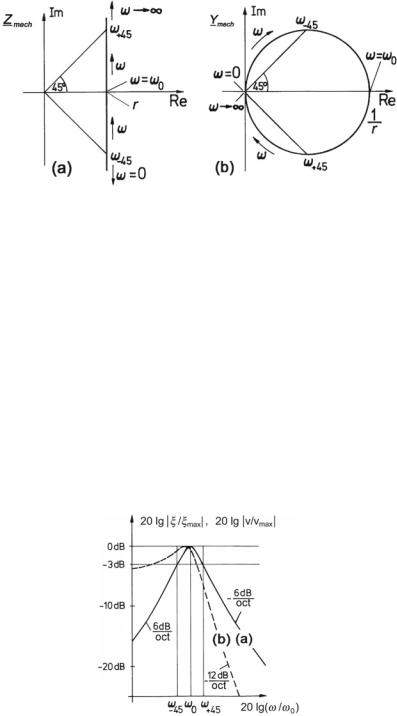
Fig. 2.4 Trajectories of mechanic impedance/admittance in the complex Z and Y planes as functions of angular frequency. (a) Mechanic impedance. (b) Mechanic admittance (mobility)
|
F |
|
|
|
1 |
|
|
|
|
|
|
Z mech = |
|
|
= j ω m + r + |
|
|
|
|
and |
(2.25) |
||
v |
j ω n |
||||||||||
Y mech = |
|
v |
= |
1 |
|
|
|
|
. |
(2.26) |
|
|
|
|
|
|
|||||||
|
F |
1 |
|
||||||||
|
|
|
|
|
j ω m + r + |
j ω n |
|
|
|
||
Figure 2.4 illustrates the trajectories of these two quantities in the complex plane as a function of frequency. The two quantities become real at the characteristic frequency, ω0. At this frequency, the phase changes signs (jumps) from positive to negative values or vice versa.
Figure 2.5 schematically illustrates functions of ξ(ω) and v(ω) in the case of slow variations of the frequency of excitation. For simple oscillators these curves have a single peak. In this example, for a case of subcritical damping with Q ≈ 2, the exciting force is kept constant over frequency.
Fig. 2.5 Mechanic responses of a simple resonator as a function of the angular frequency for constant-amplitude forced excitation. (a) Velocity. (b) Displacement

2.4 Forced Oscillation of Parallel Mechanic Oscillators |
23 |
For the velocity curve, the two points at -3 dB correspond to the frequency ω−45 and ω45. The difference of these frequencies,
ω = ω45 − ω−45 |
(2.27) |
is termed (angular frequency) bandwidth.
The quality factor, Q, is determined by this bandwidth as
Q = |
ω0 |
(2.28) |
ω . |
√
For Q ≤ 1/ 2, a displacement resonance does not occur. The course of calculations to arrive at these functions is as follows,
F |
|
F |
1 |
|
+ r, |
|
||||||||||||||||||||
|
|
|
|
= |
|
|
|
|
|
|
|
= j ω m + |
|
|
(2.29) |
|||||||||||
v |
j ω ξ |
j ω n |
||||||||||||||||||||||||
|
|
|
|
|
|
ξ |
|
= |
|
|
1 |
|
|
|
|
, |
|
|
(2.30) |
|||||||
|
|
|
|
|
|
|
|
|
|
|
|
|
|
|
|
|||||||||||
|
|
|
|
|
F |
−ω2m + n1 + j ω r |
|
|||||||||||||||||||
| ξ | |
|
|
|
|
1 |
|
|
|
|
|
|
|
||||||||||||||
|
|
|
|
= |
|
|
|
|
|
|
|
, |
(2.31) |
|||||||||||||
| |
F |
| |
|
|
|
|
|
|
|
|||||||||||||||||
|
|
( n1 − ω2m)2 + (ωr )2 |
||||||||||||||||||||||||
|
|
| v | |
= |
|
1 |
|
|
|
. |
|
(2.32) |
|||||||||||||||
|
|
| F | |
|
|
|
|
|
|
|
|
|
|
|
|||||||||||||
|
|
|
|
|
|
|
|
1 |
|
|
|
|
|
|||||||||||||
|
|
|
|
|
|
|
(ωm − |
)2 + r 2 |
|
|
||||||||||||||||
|
|
|
|
|
|
|
ωn |
|
|
|||||||||||||||||
Note that the phase of the velocity, v, is decreasing and passes zero at ω0, while the phase of the displacement, ξ, is also decreasing but goes through −π/2 at this point— see Fig. 2.6. Furthermore, the position of the peak for the |v(ω)| curve is precisely at the characteristic frequency, while the peak of the |ξ(ω)| curve lies slightly lower— the higher the damping, the lower the frequency at this peak! Hence, this peak is called the resonance. Consequently, it should be distinguished appropriately between the terms resonance frequency and characteristic frequency.
Figure 2.6 shows the resonance curves for the velocity in a slightly different way to illustrate the role of the Q-factor concerning the form of these curves. The resonance peak becomes higher and more narrow with increasing Q. This is the reason that Q is termed sharpness-of-resonance factor, besides quality factor.