


10 |
|
|
|
|
|
|
|
|
1 |
Introduction |
|
Table 1.3 Frequencies versus corresponding wavelengths in air |
|
|
|
|
|||||||
|
|
|
|
|
|
|
|
|
|
|
|
Octave-center |
16 |
32 |
63 |
125 |
250 |
500 |
1k |
2k |
4k |
8k |
16k |
frequency [Hz] |
|
|
|
|
|
|
|
|
|
|
|
|
|
|
|
|
|
|
|
|
|
|
|
Wave length |
20 |
10 |
5 |
2.5 |
1.25 |
0.63 |
0.32 |
0.16 |
0.08 |
0.04 |
0.02 |
in air [m] |
|
|
|
|
|
|
|
|
|
|
|
|
|
|
|
|
|
|
|
|
|
|
|
Ψsemitone = 12 ld ( f2/ f1), |
in [semitone] |
Ψcent = 1200 ld ( f2/ f1), |
in [cent] |
The first two logarithmic frequency intervals are often called octave and thirdoctave. The equations, Ψoct = 1, indicates one octave. Ψ3rd oct = 1 indicates one third of an octave. The four logarithmic frequency intervals have the following relationship to each other, 1 oct = 3·3rd oct = 12 semitone = 1200 cent.
A bandpass filter, which is a filter that filters out certain regions from a frequency spectrum and blocks the rest, is called octave filter when the difference between the upper and lower limiting frequencies of the pass-band amounts to one octave. Accordingly, there are, for example, third-octave filters. Note that the specification of limiting frequencies is task-specific.
In communication engineering, decades (10 : 1) are sometimes preferred to octaves (2 : 1). Conversion is as follows: 1 oct ≈ 0.3 dec or 1 dec ≈ 3.3 oct.
Wavelength, λ, and frequency, f , of an acoustic wave are linked by the relationship c = λ · f . In air we have c ≈ 340 m/s. In Table 1.3, a series of frequencies is presented with their corresponding wavelengths in air. The series is taken from a standardized octave series that is recommended for use in engineering acoustics.
In the audible frequency range, the wavelengths extend from a few centimeters to many meters. Because radiation, propagation, and reception of waves are characterized by the linear dimension of reflecting surfaces relative to the wavelength, a wide variety of different effects, including reflection, scattering, and diffraction, are experienced in acoustics.
1.7 Double-Logarithmic Plots
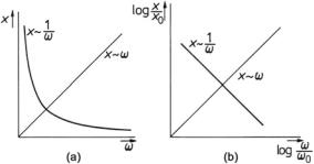
By plotting levels over logarithmic frequency intervals, one obtains a doublelogarithmic graphic representation of the original quantities. This way of plotting has some advantages over linear representations and is quite popular in acoustics.7 Figure 1.2a presents an example of a linear representation, and Fig. 1.2b shows its corresponding double-logarithmic plot.
In double-logarithmic plots, all functions that are proportional to ω y appear as straight lines since
7 In network theory, double-logarithmic graphic representations are known as Bode diagrams.
1.7 Double-Logarithmic Plots |
11 |
Fig. 1.2 Different representations of frequency functions. (a) Linear. (b) Double-logarithmic
x = a ω y → log x = log a + y log |
ω . |
(1.13) |
For integer potencies, y = ± n with n = 1, 2, 3, . . ., |
we arrive |
at slopes of |
± n · 6 dB/oct for sound pressure, displacement, and particle velocity, and of ± n · 3 dB/oct for power and intensity. For decades the respective values are ≈20 dB/dec and ≈10 dB/dec.
Functions with different potency of ω are quite frequent in acoustics. This results from the fact that differential equations of different degrees are used to describe vibrations and waves. The slope of the lines in the plot helps to estimate the order of the underlying oscillation processes.
1.8 Exercises
Recapitulation of Complex Notation
Problem 1.1 Use Euler’s formula to derive a real-valued sinusoidal expression for z(t) from the complex-valued exponential time function. Euler’s formula reads as follows,
|
= ˆ |
|
z |
z e j (ω t+φ). |
(1.14) |
Problem 1.2 Given a sinusoidal electric voltage signal
u(t) = uˆ cos(ω t + φ) , |
(1.15) |
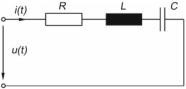
find the electric current, i(t), in Fig. 1.3 by applying complex notation.
Problem 1.3 For experimental determination of the mechanic impedance, Z mech, of a solid material (object) in practice, one may excite the object under test by
12 |
1 Introduction |
Fig. 1.3 Serial electric circuit consisting of resistance, R, inductance, L, and capacitance, C
applying a sinusoidal |
force, F(t) = |
F cos( |
ω |
t |
+ φF |
), and measuring the accelera- |
|
ˆ |
|
|
tion, a(t) = aˆ cos(ω t + φa), at the point of interest.
Determine the mechanic impedance, Z mech, at this point via the given excitation and the resulting acceleration responses.
Problem 1.4 Given a reference pressure of p0, rms = 20 µN/m2,
(a)Find the sound-pressure level of prms = 0.1 N/m2 and prms = 102 N/m2, respectively.
(b)Evaluate the sound-pressure levels for the case that the sound pressures under (a) are three-times larger.
Problem 1.5 Which frequency ratios and which logarithmic frequency intervals are represented by three semitones and by twelve semitones?
Problem 1.6Ψ |
oct = ld ( f2/ f1), |
oct |
] |
|
|
in [1 |
|
||
Ψ1/3rd oct = 3 ld ( f2/ f1), |
in [ 3 |
oct] |
||
Ψsemitone = 12 ld ( f2/ f1), |
in [semitone] |
|||
Ψcent = 1200 ld ( f2/ f1), |
in [cent] |
|||
Given the third-octave-band interval, Ψ3rd oct = 1, and the octave-band interval,
Ψoct = 1.
–Determine the corresponding frequency ratios, ( f2/ f1)3rd oct and ( f2/ f1)oct.
–Use these frequency ratios to find the two limiting frequencies, that is, the lower limiting and the upper limiting frequency, fl, and fu, of a 3rd-octave band and of an octave band with a given center frequency of fc.
Problem 1.7 Establish a table for the addition of sound-pressure levels of multiple incoherent sound sources of equal level and equal distance to the receiving point. The number of sound sources is 1, 2, 3, 4, 5, 6, 8, or 10, repectively.
1.8 Exercises |
13 |
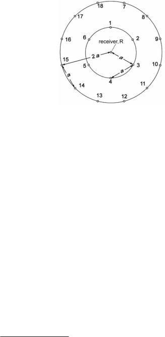
Fig. 1.4 Multiple sound sources of equal intensity in an open-space office
Problem 1.8 In an open-space office there are multiple noise sources (talking persons), spatially distributed as shown in Fig. 1.4. Sources 1–6 are located along a circle of radius a around the receiver, R, with a mutual distance of a between them. Sources 7–18 are located apart from each other by, again, a distance of a and along a circle of radius 2 a around the receiver. The sound-pressure level is assumed to decrease by 5 dB when doubling the distance in this particular space.8
With the sound-pressure level being 65 dB(A) at a 1-m distance from any single source (talker) for all directions, find the sound-pressure level at the receiver as a function of the number of sound sources (a = 4 m).
8 This, by the way, indicates that the sound-field in the specific space given here is not an entirely free field. For a perfectly free-field, we would expect a decrease of 6 dB/distance-doubling for spherical sound sources (4.25).