

196 12 Geometric Acoustics and Diffuse Sound Fields
The rays transport this energy to the wall on an average of n times per second, that
is |
|
|
|
|
W c |
|
|
|
|
|
|
A c |
|
||
|
|
W |
|
|
|
|
|
|
|
|
|
|
|||
|
n |
V |
= |
d |
A |
· |
1 s, with |
n |
= |
|
. |
(12.21) |
|||
|
4 |
|
|||||||||||||
|
|
|
d |
|
|
|
|
|
4 V |
|
|||||
This leads to the expression for the mean free-path length as
|
|
|
c |
|
4 V |
|
||
l = |
|
|
|
= |
|
. |
(12.22) |
|
|
|
|
A |
|||||
|
n |
|||||||
12.5 Reverberation-Time Formulas
When inserting the average reflection density, n , and the average degree of absorption, α, into (12.5), which describes the decay of a multiply reflected wave bundle— see Sect. 12.2—we obtain the following expression for the time-dependency of the energy density in the diffuse sound field,
|
|
|
|
|
|
|
|
|
|
|
|
0) e [ |
A c |
ln(1− |
|
) t] . |
|
|
W |
(t) |
|
W |
(t) |
|
W |
(t |
|
|
(12.23) |
||||||||
= |
= |
= |
α |
|||||||||||||||
4 V |
||||||||||||||||||
|
d |
|
|
ray |
|
|
d |
|
|
|
|
|
|
|
In practice, we compute an average degree of absorption as follows,
α = i Ai αi , (12.24)
i Ai
where αi is the individual absorption of sub-area Ai .
According to Sabine, the time span required for the energy density to decrease to one millionth of its initial value, that is, 10−6 or –60 dB, respectively, is called the reverberation time, T60. Inserting this reverberation time into (12.23) brings us to
10−6 W |
|
(t |
|
0) |
|
W |
|
(t |
|
0) e [ |
A c |
ln(1− |
|
) T60 ] . |
(12.25) |
|
= |
= |
= |
α |
|||||||||||||
4 V |
||||||||||||||||
|
d |
|
|
|
d |
|
|
|
|
|
|
|
In air under normal condition, that is, 20 ◦C temperature, 1000 hPa static pressure, and 50% humidity, the sound speed, c, is about 340 m/s. Using this value and solving for T60 in (12.25), we obtain
T60 = 13.8 |
4V |
≈ 0.163 · |
s |
V |
(12.26) |
|||||||
|
|
|
|
|
|
|
|
|
, |
|||
−ln(1 − |
|
) A c |
m |
−ln(1 − |
|
) A |
||||||
α |
α |
|||||||||||
an expression that is known as Eyring’s reverberation formula.
12.5 Reverberation-Time Formulas |
197 |
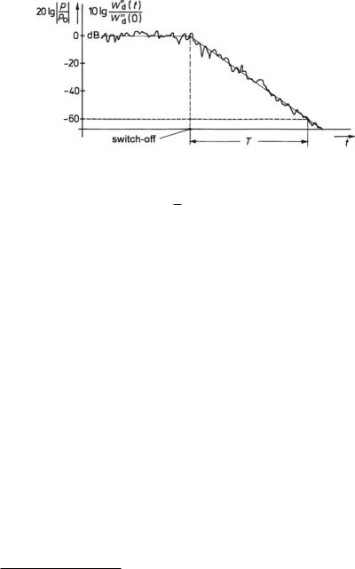
Fig. 12.12 Time trace of a reverberant noise sound after being switched off
For small amounts of absorption, α 1, this formula simplifies to
T60 = 13.8 |
4V |
≈ 0.163 · |
s |
V |
(12.27) |
|||||
|
|
|
|
|
|
|
, |
|||
|
A c |
|
m |
|
A |
|||||
α |
α |
|||||||||
which is preferred in practice and known as Sabine’s reverberation formula. There are different ways of measuring the reverberation time, including the
switch-off method, and the integrated-impulse-response method.
Using the switch-off method, a room is excited with a noise source until a steadystate energy-density level is reached. Then the sound source is switched off, and the sound energy-density level, respectively, the sound-pressure level, is recorded as a function of time, producing an energy-density time function like the one graphically presented in Fig. 12.12. The recorded graph is the so-called energy time curve.
The time interval between switching-off the source and the instant at which the sound-energy level has decreased by 60 dB is taken as the reverberation time, T60. Besides T60 other reverberation quantities are in use referring to less dynamic level ranges, for example, T30, which relates to a decay of 30 dB, yet extrapolated to a decay of 60 dB.6 In practice, the decay range is often taken from –5 dB downwards.
The switch-off method has the disadvantage that the state of the sound field is not clearly defined at the switch-off instant because the exiting noise is of stochastic nature. The measured decay traces, D(t), thus vary between trials.
This statistical uncertainty is overcome with the integrated-impulse-response method, also known as Schroeder’s method. Here the excitation is accomplished with a distinct sound impulse.7
6 Besides T30 and T60, the early-decay time, Tedt , is a relevant decay parameter, which is defined by the slope of the first 10-dB energy decay after the switch off, but then extrapolated linearly to a decay of 60 dB. Tedt is considered to correlate well with the instantaneous perception of reverberance.
7 There also exist advanced correlation methods using pseudo-random or swipe-sine excitations to determine the impulse responses experimentally.
198 |
12 Geometric Acoustics and Diffuse Sound Fields |
For this method, we first record the room impulse response, h(t), and then perform the following integration of it,
D(t) = |
∞ |
h2(τ ) dτ = |
tL |
h2(τ ) dτ , |
(12.28) |
t |
t |
where h(t) is determined between the sound source and a microphone in the room concerned. h(t) extends to a finite temporal length,8 tL. The integral in (12.28) is called Schroeder integration, carried out merely up to the time limit, tL, for example, with a value adjusted to 1–1.5 times of the expected reverberation time.
Considering the theory of diffuse sound field predicts that the diffuse-field assumption is sufficiently valid within the frequency range that the geometrical acoustics is applicable when the following conditions are met.
–Sound absorption is well distributed about the boundaries of the room.
–The shape of the room is irregular and, in particular, focusing elements are avoided.
–Total sound absorption is small or moderate. A good check is whether the ratio of room volume and equivalent absorbent area—see next paragraph—is not too small, usually > 1 m.
The Equivalent Absorbent Area
The following expression,9
A = |
|
A with |
|
1, |
(12.29) |
α |
α |
is understood to be a conceptual area with a unit degree of absorption, that is 100% of absorption or α = 1, representing the total absorption present in the room. This conceptual area is called equivalent absorbent area.
If there are partial areas at the boundary of a room, each with an individual absorption value of αi, then the equivalent absorbent area is defined to be
8To determine frequency-dependent reverberation times, band-pass filters, for example, with octave bandwidth or third-octave bandwidth, are applied to filter the broadband room impulse response, h(t), before Schroeder’s integration.
9For moderate α values ranging approximately 0 < α < 0.5, the absorption term in Eyring formula yields a more general expression for the equivalent absorption area, A = −ln(1 − α) A.

12.5 Reverberation-Time Formulas |
199 |
|
|
|
|
|
|
|
|
|
air V m−1 , |
|
|
||||
A |
|
Ai |
|
i |
|
8 |
|
(12.30) |
|||||||
|
α |
|
α |
||||||||||||
|
|
|
|
|
|
|
|
|
|
|
|
|
|
|
|
|
= |
i |
+ |
|
|
[ |
|
] |
|
|
|||||
|
|
|
|
|
correction |
|
|
|
|||||||
|
|
|
|
|
|
|
|
|
|
|
|||||
where Ai are the individual areas with individual |
degrees of absorption |
|
i. The |
||||||||||||
α |
|||||||||||||||
correction component in the formula, not derived here, is only used to account for dissipation in the transmission medium of large rooms. Values of αair are given in Table 11.1.
12.6 Application of Diffuse Sound Fields
This section introduces three frequently used applications of the diffuse-sound-field model.
Reverberation-Time Acoustics
The reverberation time, T60, estimated with either Eyring’s or Sabine’s formula, is one of various relevant parameters of the quality-of-the-acoustics of spaces, which includes, among other things, their suitability for specific performances.
Table 12.1 presents preferred values of T60 for various performance styles. The values are drawn from the literature and refer to the 500–1000 Hz range. Many acoustical consultants consider a moderate increase toward low frequencies as adequate because it is said to increase the listeners’ sense of warmth and envelopment. Yet, there is also dissenting opinion, arguing that an increase of reverberation toward low frequencies affects articulation accuracy. This is an issue, particularly, in spaces for sound recordings such as recording studios.
The following guidance holds for speech. A too-short reverberation time produces high intelligibility but also increases the effort required from the speaker. If T60 is too long, auditory smearing takes place and deteriorates intelligibility. 0.8–1.0 s is a reasonable compromise for speech running at normal speed, that is, roughly a rate of 50 syllables/minute.
Reverberation time is undoubtedly a relevant parameter of room-acoustic quality but certainly not the only one. Proper guidance of early reflections and avoidance of echoes are at least as relevant.
Table 12.1 |
Reverberation times |
|
|
|
|
Speech |
|
Chamber music |
Opera houses |
Concert halls |
Organ music |
|
|
|
|
|
|
0.8–1.0 s |
|
1.4–1.6 s |
1.5–1.7 s |
1.9–2.2 s |
2.5 s and more |
|
|
|
|
|
|
200 |
12 Geometric Acoustics and Diffuse Sound Fields |
Measurement of Random-Incidence Absorption
Random-incidence absorption measurements are conducted in reverberation chambers. These are special spaces where a diffuse sound field is be realized by using highly reflective, obliquely oriented walls and panels.10
The equivalent absorbent area, Aα1 , of the empty chamber is be determined beforehand, usually by a reverberation-time measurement for T1 . With a sample of the material to be measured in the chamber, the reverberation-time measurement is then repeated. Using the measured reverberation-time, T2 , then, the equivalent absorbent area of the chamber including the sample is,
Aα2 = 0.163 |
s |
V |
(12.31) |
|||
|
|
|
|
. |
||
|
m |
Tα2 |
||||
Consequently, the equivalent absorption area of the sample results in
A ,sample = A sample |
|
sample = A2 − A1 , |
(12.32) |
α |
where A sample is the sample size under test. The random-incidence degree of absorption, α sample, results as follows,
|
|
s |
|
1 |
|
|
|||||
|
|
V |
1 |
|
|
||||||
α |
sample = 0.163 |
|
|
|
|
|
|
− |
|
. |
(12.33) |
m |
A sample |
T2 |
T1 |
||||||||
Measurement of the Total Power of a Sound Source
For measurements of the emitted power of sound sources, diffuse sound fields in reverberation chambers are in use. To this end, the source is brought into the chamber and operated to transmit ongoing sounds.
The sound power transmitted by the source and the sound power absorbed by the equivalent absorbent area of the reverberation chamber reaches a stationary balance as follows.11
|
|
|
|
|
|
|
|
|
Aα W c |
|
|
|
Id |
|
p2 |
|
||||||
|
|
|
|
|
|
|
|
|
|
|
|
|||||||||||
|
Psource |
|
|
|
|
|
d |
|
with W |
|
|
|
= |
rms |
. |
(12.34) |
||||||
|
= |
|
|
|
|
|
|
|
= c |
|
||||||||||||
|
|
|
|
|
|
|
4 |
|
|
|
|
d |
c2 |
|
||||||||
|
|
|
|
|
|
|
||||||||||||||||
introduced |
|
|
|
|
|
|
|
|
|
|
|
|
|
|
||||||||
|
|
|
|
|
|
|
|
|
|
|
|
|
|
|
|
|||||||
absorbed
The power of the sound source, consequently, is
10To measure α for perpendicular sound incidence only, measuring tubes are applied—see Sect. 7.6. Note that α is then termed normal-incidence absorption, α .
11p rms is the rms-value of sound pressure, p—see Sect. 16.4 for its definition.
12.6 Application of Diffuse Sound Fields |
201 |
Aα |
|
Psource = p2rms 4 c . |
(12.35) |
The following rules are useful when performing the measurements. A sufficient number of measuring points must be well-distributed across the room but not too close to walls or corners because there is no guarantee for full incoherence of incoming and reflected sounds in such locations. These positions may thus result in too high measured values.
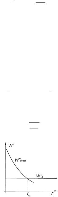
The Critical Radius
A stationary, diffuse sound field has the same average energy density, Wd , everywhere in space. Close to a sound source, however, the energy density of the direct sound is much higher. The situation is depicted in Fig. 12.13.
The critical radius is the distance from a 0th-order spherical source where the direct and diffuse energy densities are just equal. Equality of the two energy densities is given at
W |
|
= |
|
Psource |
|
1 |
! |
W |
|
= |
|
4 Psource |
|
1 |
, |
(12.36) |
|||||||||
|
|
4 π r2 |
c |
|
|
A |
|
|
|
|
c |
||||||||||||||
|
direct |
|
|
= |
|
d |
|
|
α |
|
|
||||||||||||||
|
|
|
|
|
|
|
|
|
|
|
|
|
|
|
|
|
|
|
|
||||||
|
|
|
|
|
Idirect |
|
|
|
|
|
|
|
|
|
|
|
|
|
|||||||
|
|
|
|
|
|
|
|
|
|
|
|
I diffuse |
|
|
|
||||||||||
which leads to the critical radius as follows,
|
|
|
rc = |
Aα |
(12.37) |
16 π . |
Fig. 12.13 The critical radius—the equilibrium of directand diffuse-field energy densities with a 0th-order spherical source