

154 |
10 Piston Membranes, Diffraction and Scattering |
10.1 The Rayleigh Integral
A small vibrating piston results in a 1st-order spherical sound field—see Fig. 9.6b. However, when hydrodynamic shorting between the front and back of the baffle is prohibited by placing this piston into an infinitely extended, plane and rigid baffle, we get a hemispherical sound field of 0th order radiating into half of the space— illustrated in Fig. 10.1. The hemispherical sound field is
|
→(r) = |
j ω |
e−jβr |
|
(10.1) |
||||
p |
|
|
q |
0 |
|
, |
|||
2 π |
r |
||||||||
|
|
|
|
||||||
where 2π is the spatial angle of a hemisphere. Assuming that the baffle is flat, this sound field has no normal components in the baffle’s plane, and, therefore, the baffle cannot cause any reflection or diffraction.
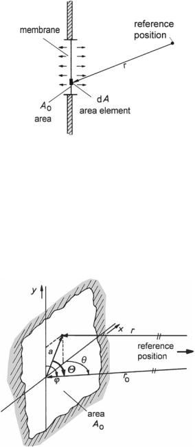
Now consider an oscillating membrane with an area A0 in this infinitely extended, flat and plane baffle where all area elements oscillate perpendicularly to the area. We consider this arrangement the superposition of an infinite number of adjacent monopoles, dq 0 = v d A,—depicted in Fig. 10.2. The total sound pressure at an observation point is found by superposition of these monopoles, vis,
p |
→(r) = |
j ω |
|
v(x, y) |
e−jβr |
d A . |
(10.2) |
|
2 π |
A0 |
r |
||||||
|
|
|
|
In acoustics, this integral is usually called Rayleigh integral. It is valid at all distances from the membrane.
It is worth noting that v (x, y) needs not be the same everywhere on the membrane. Its value may depend on the position of the membrane. A finite area A0 is required for the Rayleigh integral to converge without additional assumptions, such as propagation losses in the medium. Further, no obstacles are admitted in the hemisphere concerned.
Fig. 10.1 Hemispherical sound field, originating from a point source in a flat and rigid baffle
10.2 Fraunhofer’s Approximation |
155 |
Fig. 10.2 Sound field in front of a membrane in a flat and rigid baffle
10.2 Fraunhofer’s Approximation
Fraunhofer’s approximation applies when the distance from the reference point to the membrane is very large compared to the linear dimensions of the radiating membrane. Figure 10.3 depicts the situation to be discussed.
The quantity, r0, is the distance from the reference point to any position on the membrane within the area A0. That position is preferably the membrane’s center of
Fig. 10.3 Fraunhofer’s approximation
156 |
10 Piston Membranes, Diffraction and Scattering |
gravity. The angle between r and r0 is very small, and the two lines are practically parallel. The following linear approximation is thus applicable,
r ≈ r0 − a cos Θ , |
(10.3) |
where Θ is the angle between r0 and a. |
|
We express this setting in Cartesian coordinates as |
|
r ≈ r0 − x cos θ − y cos ϕ , |
(10.4) |
where θ is the angle between r0 and the x-axis, and ϕ is the angle between r0 and the y-axis. The factor 1/r is brought out in front of the integral because 1/r ≈ 1/r0—as we saw in Sect. 9.5. Thus, we get
p |
→(r, θ, ϕ) ≈ |
j ω e−jβr0 |
× |
|
2 π r0 |
||||
|
+∞ +∞
v(x, y) e j(β cos θ)x e j(β cos ϕ)y dx dy . (10.5)
−∞ −∞
This expression is again isomorphic to a Fourier transform. It is actually a twodimensional, spatial Fourier transform, where β cos θ is the phase coefficient in x- direction, and β cos ϕ is the phase coefficient in y-direction. Recall that β = 2π/λ.
10.3 The Far-Field of Piston Membranes
This section deals with the sound field produced by rigid membranes, so-called piston membranes, in infinitely extended, rigid, flat baffles. In other words, we speak of baffled pistons with identical v (x, y) everywhere on the piston. Such piston membranes qualify as appropriate models for loudspeakers in large baffles as long as the membranes of the loudspeakers vibrate in phase.
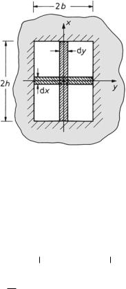
Rectangular Piston Membranes
The computation of the sound field of a rectangular piston membrane in an infinitely extended, rigid, flat baffle is feasible with Fraunhofer’s approximation according to Fig. 10.4. By symbolizing the constant factors left of the integral as C 1 or C 2, respectively, we write Fraunhofer’s approximation and its Fourier transform as follows,
10.3 The Far-Field of Piston Membranes |
157 |
Fig. 10.4 Rectangular membrane
p →(r, θ, ϕ) = C 1 |
+b |
|
+h |
v e j(β cos θ)x e j(β cos ϕ)y dx dy |
(10.6) |
|||||||||||||||||
b |
|
h |
||||||||||||||||||||
|
|
|
|
− |
|
|
− |
|
|
|
|
|
|
|
|
|
|
|
|
|
|
|
|
|
|
= C 2 |
+h |
|
|
|
|
|
|
|
|
+b |
|
|
|
|
|
|
|
|
|
|
|
|
e j(β cos θ)x dx |
e j(β cos ϕ)y dy , |
(10.7) |
|||||||||||||||||
|
|
|
|
−h |
|
|
|
|
|
|
|
|
−b |
|
|
|
|
|
|
|
|
|
|
|
|
|
|
|
◦ |
|
|
|
|
|
|
|
|
◦ |
|
||||||
|
|
|
|
|
|
• |
|
|
|
|
|
|
|
|
• |
|
||||||
|
p |
→(r, θ, ϕ) ◦ |
• C 2 2h si (h β cos θ) 2b si (b β cos ϕ) . |
(10.8) |
||||||||||||||||||
|
|
|
||||||||||||||||||||
|
|
|
|
|
|
|
|
|
|
|
|
|
|
|
|
|
|
|
|
|||
|
|
|
|
|
|
|
|
|
Γ (θ) |
|
|
|
Γ (ϕ) |
|
||||||||
Because each of the two integrals is a one-dimensional Fourier integral, the integration is subject to well-known rules. The result of the integration is (10.8), where the first term on the right-hand side includes the directional characteristic concerning θ, and the second one for ϕ. The total two-dimensional directional characteristic is formed by multiplying the two one-dimensional characteristics. Each of them represents a continuously loaded line array, one on the x-axis, and another on the y-axis. Thus, we get
Γ (θ, ϕ) = Γ (θ) Γ (ϕ) . |
(10.9) |
The third dimension, r, is not considered because the derivation above only deals with the sound field far away from the membrane.
Circular Piston Membranes
The calculation of circular pistons is slightly more complicated and requires a transformation into polar coordinates—illustrated in Fig. 10.5. The result of the calculation is given below,