

5.2 Magnetodynamic Sound Emitters and Receivers |
73 |
range. The following two construction features distinguish cardioid microphones. Both of them decrease the proximity effect—compare Sect. 4.7.
–The variable-distance principle uses delay lines with different effective lengths for different frequencies to increase the driving force at low frequencies.
–The double-path principle uses two transducers with different delay lines, one for the high frequencies and one for the low. The two transducers are connected by an appropriate cross-over network.
5.3The Electromagnetic Transduction Principle
The Inner Transducer
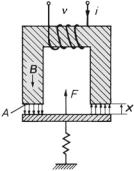
Figure 5.12 illustrates the fundamental arrangement for the inner-transducer principle. To derive the transducer equation, we compute the force on the movable armature by imagining a small virtual shift of the armature, dx.
We start with a fundamental relation from electrodynamics, Ampere’s law, which states that in an arrangement as shown in Fig. 5.12, the electric current, i, and the magnetic-flux density, B, are proportional as follows,
i ν = (B/µ0) 2 x , ν . . . |
number of turns in the coil |
(5.12) |
whereby it is assumed that the iron cores of the yoke and the movable armature are highly permeable, so that the energy of the magnetic field is concentrated in the air-gap, 2 x. Multiplication with the cross-sectional area of the air-gap, A, renders
A · i · ν = ( A · B/µ0) 2 x = (Φ/µ0) 2 x , |
(5.13) |
Φ is the magnetic flux. By inserting the definition of the inductance, L = ν Φ/ i, into (5.13), we get the inductance of our arrangement in the form of
Fig. 5.12 Electromagnet with a movable armature
74 5 Magnetic-Field Transducers
|
|
|
|
|
L = ν2 |
µ0 A |
|
|
|
|
(5.14) |
|||||||||
|
|
|
|
|
|
|
|
|
. |
|
|
|
|
|||||||
|
|
|
|
|
|
2 x |
|
|
|
|
||||||||||
Referring to (5.1) and (5.14), we now compute the contracting force as |
|
|||||||||||||||||||
|
d |
1 |
|
1 |
|
i2 ν2 |
B2 A |
|
Φ2 |
|
||||||||||
F(x) = − |
|
|
|
L(x) i2 |
= |
|
|
|
|
|
|
|
µ0 A = |
|
= |
|
. |
(5.15) |
||
dx |
2 |
2 |
2 x2 |
µ0 |
µ0 A |
|||||||||||||||
|
|
|
|
|
|
|
|
|
|
|
|
|
|
|
|
|||||
|
|
|
|
|
(B |
0 |
|
|
|
|
|
|
|
|||||||
|
|
|
|
|
|
|
|
/µ |
)2 |
|
|
|
|
|
|
|
||||
This is clearly a quadratic power law. To linearize it, we add a permanent magnetic flux, Φ−, as a magnetic bias—either by applying a permanent magnet or due to a constant current, i−. This flux is large as compared to the alternating flux, Φ , and the two result in Φ = Φ− + Φ , leading to
F(x) ≈ |
2 Φ− Φ |
= |
|
2 Φ− |
|
ν µ0 A |
, |
(5.16) |
|||||||
|
|
µ0 A |
|
|
µ0 A |
|
|
2 x |
|||||||
with |
|
|
L i |
|
= ν |
|
µ0 A |
|
|
|
|
|
|||
Φ = |
|
i . |
|
(5.17) |
|||||||||||
ν |
|
|
2 x |
|
|||||||||||
In this way, we obtain the first transducer equation, |
|
|
|
|
|||||||||||
|
F i |
≈ ν |
x − i i . |
|
|
|
(5.18) |
||||||||
|
|
|
|
|
|
Φ |
|
|
|
|
|
|
|
|
|
The second equation is easily derived by considering the equality of the inand output power in (5.9), resulting in
u i ≈ ν |
x − v i . |
(5.19) |
|
|
|
Φ |
|
Note that the permanent flux, Φ−, and the number of turns, ν, appear in the relationship for the transducer coefficient, M = (ν Φ−)/x. This means that the transducer becomes more efficient and, therefore, more sensitive with increasing magnetic bias and an increasing number of coil turns.
The Real Transducer
The equivalent circuit of the real electromagnetic transducer corresponds to the magnetodynamic transducer circuit, with the addition of one very interesting feature. The mechanic compliance is supplemented by a negative compliance called the field com-
5.3 The Electromagnetic Transduction Principle |
75 |
pliance, nf = dx/dF|i− , which results from decreasing the air-gap4. The decreasing gap increases the force attracting the armature and opposing the reversing mechanic force. For large displacements this may cause the membrane to bounce to one of the magnet poles and cling there. This is a very undesired effect that becomes more likely with increasing permanent magnetic bias—compare the solutions to problem 5.2.
5.4 Electromagnetic Sound Emitters and Receivers
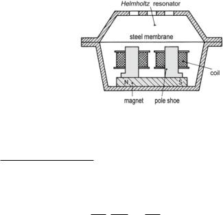
Electromagnetic transducers come in very small and efficient form. Yet, nonlinear distortions are harder to manage than with magnetodynamic transducers because of the intrinsically quadratic force law. Examples of traditional applications include telephone-receiver capsules, miniature microphones for hearing aids, pick-up transducers for record players, and free-swinging loudspeakers. An electromagnetic telephone-receiver capsule and a hearing-aid microphone are shown in Figs. 5.13 and 5.14 for historical reasons.
In the traditional telephone capsule, a Helmholtz resonator tuned to the middle of the speech spectrum is put on top of the membrane to improve the capsules sensitivity for speech signals. Note that low-frequency tuning supports membrane clinging— undesired as explained above.
Fig. 5.13 Telephone-receiver capsule
4 The field compliance is derivable by a virtual shift as follows,
|
1 |
i− = |
dF |
= |
2Φ− dΦ− |
= |
|
2Φ− −νi− µ0 A |
||||||||||
|
|
|
|
|
|
|
|
|
|
|
|
|
|
|||||
nf |
dx |
µ0 A dx |
|
µ0 A |
2x2 |
|||||||||||||
|
|
|
|
|
|
|
|
|
|
|
2 |
|
−2x |
(5.20) |
||||
|
|
|
2Φ− |
|
Φ− |
|
νΦ− |
|
|
|
M2 |
. |
||||||
= |
µ0 A −x |
= x |
|
|
µ0 Aν2 |
|
||||||||||||
|
= − L |
|||||||||||||||||
76 |
5 Magnetic-Field Transducers |
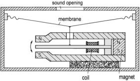
Fig. 5.14 Hearing-aid microphone
Table 5.1 Magnetization coefficients of different magnetostrictive materials
Material |
Magnetization Coefficient |
|
|
|
|
Iron |
l |
/ l = −8 · 10−6 |
Cobalt |
l |
/ l = −55 · 10−6 |
Nickel |
l |
/ l = −35 · 10−6 |
Ferrite |
l |
/ l = −100 to + 40 · 10−6 |
A special construction trick—shown in Fig. 5.14—has long been used to manufacture efficient miniature microphones. The reed is very thin. This is possible as it is not pre-magnetized. The result is a microphone that is less than 1 cm large and has a sensitivity on the order of T up ≈ 1 mV/Pa.
5.5 The Magnetostrictive Transduction Principle
Rods made of ferromagnetic material experience a variation of their lengths when exposed to magnetic fields. A common model of this effect considers the distances between the molecules as forming a fictive air-gap. Such a model leads to the same transducer equations as those of the electromagnetic transducer. The force law is intrinsically quadratic and requires linearization for transducer use.
Table 5.1 lists one-dimensional magnetization coefficients, l / l, for a number of magnetostrictive materials. A negative sign means that the rod length decreases when the material is magnetized. Yet, increases do also occur, for example, in ferrite rods. More sophisticated models than the simple air-gap model are able to explain this effect.