

56 |
4 Electromechanic and Electroacoustic Transduction |
4.7 Further Directional Characteristics
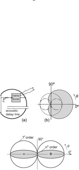
When linearly superimposing a pressure and pressure-gradient receiver, one arrives at a directional characteristic called cardioid. Figure 4.15a shows such a characteristic. The mathematical expression for it is
Γ = |
1 |
(1 + cos θ) , |
(4.27) |
2 |
where the reference direction for normalization is again the receiver axis.
There are two ways of realizing such a receiver. The first one is to arrange both receivers in practically the same position—coincident microphones—and add their output signals in phase and with the same amplitude at frontal incidence. The second one—illustrated in Fig. 4.15b—uses an acoustic delay line to guide sound from the rear side of the receiver to the back of the membrane.
Receivers that select higher-order pressure gradients from the sound field than gradient receivers with a figure-of-eight characteristic achieve even sharper spatial selectivity. The higher orders are determined according to ∂n p/∂rn and lead to directional characteristics as depicted in Fig. 4.16. These receivers are, however, even less sensitive and very frequency dependent, according to F ωn. The analytical expression for their directional characteristic is
Γ = cosn θ . |
(4.28) |
Fig. 4.15 Cardioid microphone. (a) Construction. (b) Directional characteristic
Fig. 4.16 Higher-order figure-of-eight directional characteristic
4.7 Further Directional Characteristics |
57 |
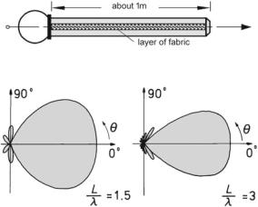
Fig. 4.17 Line microphone
Fig. 4.18 Directional characteristics of line microphones of different length
The receivers we dealt with so far were all small compared to the wavelengths considered, so that no interference takes place. We now discuss an example of a receiver that is distinctly larger than typical wavelengths. This so-called line microphone— schematically depicted in Fig. 4.17—deliberately exploits interference of incoming waves.
A line microphone is a receiver with an extremely narrow directionality, feasible for a fairly broad frequency band. It consists of a tube that is typically open at one end and fitted with a microphone at the other one. Along the tube there is a slit through which sound can enter.
Now consider the following two extreme cases.
–Sound impinges laterally, meaning that all points on the slit are excited in phase, prompting waves that all propagate to the microphone. They cancel each other out upon arrival because of their different travel distances, making the receiver insensitive to this direction.
–Sound impinges frontally. Now all waves propagate in phase to the microphone and add up there upon arrival. The receiver has its maximum sensitivity in this direction.
Figure 4.18 illustrates the complete directional characteristics for two receivers of different length. We discuss the computation of such diagrams in Sect. 9.4. Note that the slit is often covered with fabric with a flow resistance that varies along the tube. This feature compensates for losses during wave propagation in the tube.
58 |
4 Electromechanic and Electroacoustic Transduction |
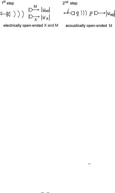
Fig. 4.19 Overview of the reversibility method for absolute transducer calibration. M … Electroacoustic coupler to be calibrated. X … Supporting transducer (reversible)
4.8 Absolute Calibration of Transducers
This section explains how the principle of reversibility is employed for the absolute calibration of an electroacoustic coupler, M. As necessary tool we need a small supporting transducer, X, which is reversible and has a spherical directional characteristic. A constant sound source is also required. At the supporting transducer we have, due to reversibility as stated in (4.16),
|
u |
|
|
= |
|
v |
|
|
and, thus, |
|
T up |
|
= |
|
|
u |
|
|
|
= |
|
|
q |
|
|
|
. |
(4.29) |
|
|
|
|
|
X |
|
|
|
|
|
|
|
||||||||||||||||||
F |
|
i |
|
|
p |
|
|
|
|
|
|
||||||||||||||||||
|
|
|
= |
|
|
|
|
= |
|
|
|
|
|
|
|
|
|
i |
= |
0 |
|
|
|
= |
|
|
|||
|
|
|
|
|
|
|
|
|
|
|
|
|
|
|
|
|
|
|
|
|
|
|
|
|
|
||||
|
|
|
|
|
|
|
|
|
|
|
|
|
|
|
|
|
|
|
|
|
|
|
|
|
|
|
|||
Figure 4.19 denotes the two steps to be taken. Firstly, both the supporting transducer and the microphone to be measured are positioned closely together (spatially coincident) in a free sound field. The output voltages of both components are measured with their electric output ports at idle. The ratio of the two voltages measured corresponds to the ratio of the sensitivities of the two transducers and is expressed as
u M1 |
= |
| T up |
|M . |
(4.30) |
||
|
uX |
|
T up |
X |
|
|
|
| |
| |
|
|
||
|
|
|
|
|
|
|
|
|
|
|
|
|
|
Secondly, we use the supporting transducer as a spherical sound source. This source is excited with a current, i, and generates a volume velocity of q. Due to the negligible power efficiency of such a source, we assume that its acoustic port is mechanically idling, that is, F = 0. This means with (4.29) that find
| q | = | T up| X | i | . |
(4.31) |
||
|
|
|
|
With the acoustic impedance, | p / q | = | Z a|, which is computable concerning the spherical sound field with the source distance known, we arrive at
| u |M2 = | p | | T up|M = | q | | Z a| | T up|M . |
(4.32) |
||||
|
|
|
|
|
|
Inserting (4.30) into (4.31) produces
4.8 Absolute Calibration of Transducers |
59 |
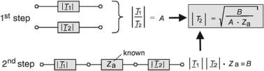
Fig. 4.20 Conceptual summary of the absolute-calibration method
| |
q |
| = | |
T up |
X |
| |
i |
| = |
|
u X |
|
|
T up |
M | |
i |
|
|
|||||||||||||
|
| |
|
|
u M1 |
|
|
|
|||||||
|
|
|
|
|
|
|
|
|
|
|
|
|
|
|
|
|
|
|
|
|
|
|
|
|
|
|
|
|
|
|
|
|
|
|
|
|
|
|
|
|
|
|
|
|
Filling this expression into (4.32) results in
| |
u |
| |
M2 |
= | |
Z a |
| |
( |
| |
T up |
M)2 |
|
u X |
|
| |
i |
| |
, |
||||||
|
|||||||||||||||||||||||
|
|
|
|
|
| |
|
u M1 |
|
|
|
|||||||||||||
|
|
|
|
|
|
|
|
|
|
|
|
|
|
|
|
|
|
|
|
|
|
|
|
|
|
|
|
|
|
|
|
|
|
|
|
|
|
|
|
|
|
|
|
|
|
|
|
|
|
|
|
|
|
|
|
|
|
|
|
|
|
|
|
|
|
|
|
|
|
|
|
|
|
|
|
| |
T up |
M |
= |
|
|
| u M1 | | u M2 | |
|
|
|
. |
|
|
|||||||
|
|
|
|
|
| Z a| |u X| | i | |
|
|
||||||||||||||||
|
|
|
|
|
| |
|
|
|
|
|
|
|
|||||||||||
| .
or
(4.33)
(4.34)
(4.35)
Note that only electric measurements are necessary to determine the sensitivity coefficient, |Tup|M , of the electroacoustic coupler in calibration. The coupler to be calibrated needs not be reversible.
An overall accuracy of 1% can be achieved with this calibration method because electric measurements are very accurate. Therefore, certified calibration laboratories apply it. The conceptual essence of the method is summarized in Fig. 4.20. The point is that by knowing the ratio and the product of two quantities, both of them are determined.
4.9 Exercises
Electromechanic and Electroacoustic Transduction
Problem 4.1 For the mechanic system shown in Fig. 4.21, construct an analog electric circuit using analogy #2. The oscillating coil is excited by a constant force, F = constant. Neglect the volume behind the coil and the radiation impedance.
Problem 4.2 Derive the directional characteristic for an arbitrary linear combination of two collocated sound sources, one with a spherical and the other one with a figure- of-eight characteristic. Sketch the following special cases: sphere, hypocardioid, cardioid, hypercardioid, figure-of-eight.
60 |
4 Electromechanic and Electroacoustic Transduction |
Fig. 4.21 Mechanic-acoustic circuit of a loudspeaker box to be converted into an equivalent electric one by analogy #2
Problem 4.3 Sketch the directional characteristic of a line microphone, that is, a microphone at the end of a narrow tube with a slit opening. Assume plane-wave sound incidence.
Problem 4.4 Pressure-gradient receivers are implemented in practice as pressuredifference receivers.
Determine the magnitude of the pressure difference as a function of frequency, given the distance, d, to the measurement point.
Problem 4.5 In a set-up for determining the sensitivity coefficient of a transducer of magnetic-field type, dedicated for measurements of structure-born sound, the magnetic-field transducer under test is rigidly connected to two other transducers, one of which is reversible. Mass and compliance of the rigid-connection elements are given.
Determine the sensitivity coefficient of the transducer under test, based solely on the electric measurements where the reversible transducer is first used as a transmitter, and then as a receiver.
Problem 4.6 Transmission systems are often mathematically represented by chain matrices.
(a)What advantages does the chain-matrix representation have?
(b)What do the matrix elements mean?
(c)Pure acoustic or electric networks for real transducers can be presented in a form as shown in Fig. 4.22. Find corresponding matrix elements.
4.9 Exercises |
61 |
Fig. 4.22 Two-port representation of acoustic and/or electric elements
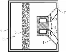
Problem 4.7 Determine the directional characteristic of a microphone as schematically depicted in Fig. 4.23.
Fig. 4.23 Schematic sketch of a microphone with rear opening p 1 and p 2 …Sound-pressure signals at the frontside and at the backside