

4.1 Electromechanic Couplers as Twoor Three-Port Elements |
|
|
|
|
|
|
45 |
||||||||||
which consequently leads to |
|
|
|
|
|
|
|
|
|
|
|
|
|
||||
|
|
|
F |
1 |
v |
F |
2 |
v |
|
|
|
|
|
|
|
|
|
F |
|
= |
|
1 − |
|
2 |
with v |
= |
v |
1 |
− |
v |
2 |
. |
(4.3) |
||
|
|
|
v1 − v 2 |
|
|||||||||||||
|
|
|
|
|
|
|
|
|
|||||||||
When the housing is fixed to the ground, as is frequently the case, v 2 |
becomes |
||||||||||||||||
zero and yields v = v 1 and F = F 1. In this case, terminal 2 may be disregarded because no power passes through it.
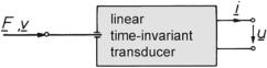
Regardless of the specific case, the essential role of the electromechanic coupler is to couple the introduced mechanic power, (1/2) F v , at one port and the provided electric power, (1/2) u i , at the other—or vice versa. Figure 4.1b illustrates the situation in form of a two-port element. This figure is the basis of our discussion for the rest of this chapter.
4.2 The Carbon Microphone—A Controlled Coupler
An important class of electromechanic couplers consists of couplers where the signalrepresenting quantities in one network, mechanic or electric, accomplish the coupling by controlling elements of the other network.
An illustrative historical example is the carbon microphone, which was an important part of telephone technology for about a century and was, during that period, the most frequently-used microphone type worldwide.
The carbon microphone is a unidirectional coupler working in the mechanic-to- electric direction. It requires a DC-power supply and behaves as an active element at its output port. It performs a power amplification on the order of 30, which is about 15 dB. This property was the main reason for its widespread use when telephone terminals had not yet other built-in amplifiers.
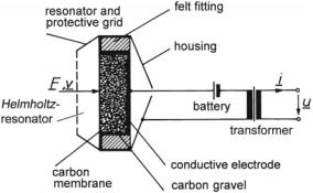
Fig. 4.3 Section view of a carbon microphone
46 |
4 Electromechanic and Electroacoustic Transduction |
Figure 4.3 illustrates a section through a carbon microphone. The electrically conducting membrane is excited by the sound-pressure impinging on it.
A conductive electrode—metal or carbone—is positioned behind the membrane, and the gap between this back electrode and the membrane is filled with fine-grain carbon gravel. Further, a Helmholtz resonator—compare Sect. 2.7—is arranged in front of the membrane to boost the sensitivity in the main frequency range of speech signals.
The electric resistance of the gravel, about 100 , varies according to the alternating pressure on it. If a DC-current is applied to this arrangement, the current superimposes on an alternating current as the resistor varies. The AC component of the current can be filtered out using a transformer—shown in Fig. 4.3. Typical carbon microphones have a sensitivity of Tup ≈ 500 mV/Pa, which corresponds to 500 mV for a 94-dB sound.
Several disadvantages should be mentioned, though. First, carbon microphones produce many upper harmonics with a power of up to 25% of the fundamental harmonic. Second, they generate quite a bit of internal noise, and, finally, they are power consuming. For these reasons, these microphones have been replaced in communication technology with electret microphones. Such microphones can be miniaturizes and realized on a silicon chip—so-called MEMS microphones —compare Sect. 6.6.
Other examples of controlled couplers are the foil-strain gauge (a controlled resistor), the piezotransistor (a pressure-sensitive transistor), and the compressed-air loudspeaker in which an electromagnetic valve controls a stream of compressed air to generate sounds of up to 160 dB.
4.3 Fundamental Equations of Electroacoustic Transducers
From an application standpoint, the most important electromechanic couplers are those where electric power is directly transformed into mechanic power, or vice versa. This class of coupler is called transducers. The term transducer is usually reserved for those couplers that can work bi-directionally and are intrinsically passive, meaning that they do not have power sources of their own. Coupling by means of transducers is retroactive because there is power flowing across the domains.
The following system of linear equations applies when the transducers are linear and time-invariant. This important case is schematically shown in Fig. 4.4.
Fig. 4.4 Schematic plot of a linear, time-invariant transducer
4.3 Fundamental Equations of Electroacoustic Transducers |
47 |
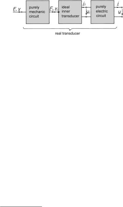
Fig. 4.5 A real transducer as a chain of three two-ports
F |
= |
A |
21 |
A |
22 |
i |
, |
(4.4) |
|
v |
|
|
A |
11 |
A |
12 |
u |
|
|
|
|
|
|
|
|
||||
where we omit the subscript from now on for simplicity. This form of the fundamental transducer equations is called the primary form. The coefficients of the transfer matrix, A ik , are called chain parameters.
We now concentrate on transducers that transform power using force effects in electromagnetic fields. In such transducers the Lorentz force is effective. This force
is expressible in general form as |
el −→ + |
|
|
−→ × |
−→ |
|
|
−→ = |
Q |
Q |
el |
(4.5) |
|||
F |
E |
|
( v |
B ) , |
|||
or, in expanded form, with l being the path of i in the B-field, |
|
||||||
−→ = |
|
−→ |
+ |
|
−→ × |
−→ |
(4.6) |
F |
(C u) E |
|
i ( l |
B ) . |
|||
Assuming the simple case |
in |
which |
the |
electric field strength, |
−→ |
||
E , and the |
|||||||
−→
magnetic-flux density, B , are constant, we draw the following principles from these equations for the forces in transducers.1
–For purely electric fields the force, F, is proportional to the voltage, u.
–For purely magnetic fields the force, F, is proportional to the current, i.
Real transducers have additional components beyond the actual energy-transducing elements. Transducers working with magnetic fields always contain an inductance, and those working with electric fields always have a capacitance. We also have to expect a resistance, representing electric power losses. On the mechanical side, mass is unavoidable. A spring is required to provide a restoring force on the oscillating mass and to compensate for gravitation, and there is usually some mechanic damping as well.
It is possible to mathematically separate the real transducer into a chain of three two-port elements—depicted in Fig. 4.5. The inner transducer can be configured as
1 In general, higher forces can be achieved with magnetic fields because the electric field-strength is limited by the danger of disruptive discharge. This is the reason why electric motors and generators usually use magnetic fields.
48 |
4 Electromechanic and Electroacoustic Transduction |
Fig. 4.6 The ideal transformer as analogy of the ideal magnetic-field transducer
ideal, that is, without any resistances, dampers, or reactances. The inner transducer cannot store energy in any way because it is lossless, and it is not directly accessible from outside. The complex power at its ports results as
F i v i = u i i i . |
(4.7) |
In the following, we derive the fundamental equations for inner transducers based on either magnetic or electric fields.
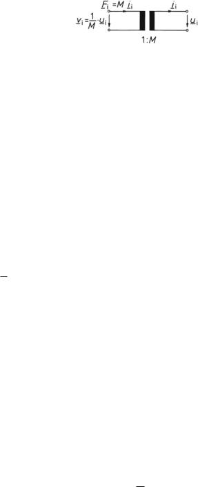
As noted above, F and v are proportional in magnetic-field transducers. The proportionality coefficient, M, is a real constant and specific to a particular transducer. With the movable component blocked, meaning v i = 0, and the electric port cut short, meaning u i = 0, we measure a force, F i, when applying a current, i i, as follows,
F i = M i i . |
(4.8) |
Since energy is neither lost nor stored in the inner transducer, the power at the two ports is identical by definition. Consequently, we know the relationship between v i and u i when F i and i i are zero, namely,
|
|
v i = |
1 |
u i |
. |
|
(4.9) |
|
|
|
M |
|
|||||
A combination of the two yields |
|
|
|
|
|
|
|
|
v |
|
= |
1/0M |
0 |
u |
. |
|
|
Fii |
M |
i ii |
(4.10) |
|||||
By applying the electromechanic analogy # 2, we identify the ideal transformer as analogy of the magnetic transducer shown in Fig. 4.6.
Electric-field transducers show proportionality of F and u. The proportionality coefficient, N , is again a real constant, and specific to a particular transducer. With
the movable component fixed, such that vi = 0, the equation is |
|
F i = N u i , |
(4.11) |
and, due to the identity of the power at the two ports, it follows that
v i = |
1 |
(4.12) |
N i i , |