

- •Contents
- •Acknowledgments
- •Preface
- •What a Crossover Does
- •Why a Crossover Is Necessary
- •Beaming and Lobing
- •Passive Crossovers
- •Active Crossover Applications
- •Bi-Amping and Bi-Wiring
- •Loudspeaker Cables
- •The Advantages and Disadvantages of Active Crossovers
- •The Advantages of Active Crossovers
- •Some Illusory Advantages of Active Crossovers
- •The Disadvantages of Active Crossovers
- •The Next Step in Hi-Fi
- •Active Crossover Systems
- •Matching Crossovers and Loudspeakers
- •A Modest Proposal: Popularising Active Crossovers
- •Multi-Way Connectors
- •Subjectivism
- •Sealed-Box Loudspeakers
- •Reflex (Ported) Loudspeakers
- •Auxiliary Bass Radiator (ABR) Loudspeakers
- •Transmission Line Loudspeakers
- •Horn Loudspeakers
- •Electrostatic Loudspeakers
- •Ribbon Loudspeakers
- •Electromagnetic Planar Loudspeakers
- •Air-Motion Transformers
- •Plasma Arc Loudspeakers
- •The Rotary Woofer
- •MTM Tweeter-Mid Configurations (d’Appolito)
- •Vertical Line Arrays
- •Line Array Amplitude Tapering
- •Line Array Frequency Tapering
- •CBT Line Arrays
- •Diffraction
- •Sound Absorption in Air
- •Modulation Distortion
- •Drive Unit Distortion
- •Doppler Distortion
- •Further Reading on Loudspeaker Design
- •General Crossover Requirements
- •1 Adequate Flatness of Summed Amplitude/Frequency Response On-Axis
- •2 Sufficiently Steep Roll-Off Slopes Between the Filter Outputs
- •3 Acceptable Polar Response
- •4 Acceptable Phase Response
- •5 Acceptable Group Delay Behaviour
- •Further Requirements for Active Crossovers
- •1 Negligible Extra Noise
- •2 Negligible Impairment of System Headroom
- •3 Negligible Extra Distortion
- •4 Negligible Impairment of Frequency Response
- •5 Negligible Impairment of Reliability
- •Linear Phase
- •Minimum Phase
- •Absolute Phase
- •Phase Perception
- •Target Functions
- •All-Pole and Non-All-Pole Crossovers
- •Symmetric and Asymmetric Crossovers
- •Allpass and Constant-Power Crossovers
- •Constant-Voltage Crossovers
- •First-Order Crossovers
- •First-Order Solen Split Crossover
- •First-Order Crossovers: 3-Way
- •Second-Order Crossovers
- •Second-Order Butterworth Crossover
- •Second-Order Linkwitz-Riley Crossover
- •Second-Order Bessel Crossover
- •Second-Order 1.0 dB-Chebyshev Crossover
- •Third-Order Crossovers
- •Third-Order Butterworth Crossover
- •Third-Order Linkwitz-Riley Crossover
- •Third-Order Bessel Crossover
- •Third-Order 1.0 dB-Chebyshev Crossover
- •Fourth-Order Crossovers
- •Fourth-Order Butterworth Crossover
- •Fourth-Order Linkwitz-Riley Crossover
- •Fourth-Order Bessel Crossover
- •Fourth-Order 1.0 dB-Chebyshev Crossover
- •Fourth-Order Linear-Phase Crossover
- •Fourth-Order Gaussian Crossover
- •Fourth-Order Legendre Crossover
- •Higher-Order Crossovers
- •Determining Frequency Offsets
- •Filler-Driver Crossovers
- •The Duelund Crossover
- •Crossover Topology
- •Crossover Conclusions
- •Elliptical Filter Crossovers
- •Neville Thiele MethodTM (NTM) Crossovers
- •Subtractive Crossovers
- •First-Order Subtractive Crossovers
- •Second-Order Butterworth Subtractive Crossovers
- •Third-Order Butterworth Subtractive Crossovers
- •Fourth-Order Butterworth Subtractive Crossovers
- •Subtractive Crossovers With Time Delays
- •Performing the Subtraction
- •Active Filters
- •Lowpass Filters
- •Highpass Filters
- •Bandpass Filters
- •Notch Filters
- •Allpass Filters
- •All-Stop Filters
- •Brickwall Filters
- •The Order of a Filter
- •Filter Cutoff Frequencies and Characteristic Frequencies
- •First-Order Filters
- •Second-Order and Higher-Order Filters
- •Filter Characteristics
- •Amplitude Peaking and Q
- •Butterworth Filters
- •Linkwitz-Riley Filters
- •Bessel Filters
- •Chebyshev Filters
- •1 dB-Chebyshev Lowpass Filter
- •3 dB-Chebyshev Lowpass Filter
- •Higher-Order Filters
- •Butterworth Filters up to 8th-Order
- •Linkwitz-Riley Filters up to 8th-Order
- •Bessel Filters up to 8th-Order
- •Chebyshev Filters up to 8th-Order
- •More Complex Filters—Adding Zeros
- •Inverse Chebyshev Filters (Chebyshev Type II)
- •Elliptical Filters (Cauer Filters)
- •Some Lesser-Known Filter Characteristics
- •Transitional Filters
- •Linear-Phase Filters
- •Gaussian Filters
- •Legendre-Papoulis Filters
- •Laguerre Filters
- •Synchronous Filters
- •Other Filter Characteristics
- •Designing Real Filters
- •Component Sensitivity
- •First-Order Lowpass Filters
- •Second-Order Filters
- •Sallen & Key 2nd-Order Lowpass Filters
- •Sallen & Key Lowpass Filter Components
- •Sallen & Key 2nd-Order Lowpass: Unity Gain
- •Sallen & Key 2nd-Order Lowpass Unity Gain: Component Sensitivity
- •Filter Frequency Scaling
- •Sallen & Key 2nd-Order Lowpass: Equal Capacitor
- •Sallen & Key 2nd-Order Lowpass Equal-C: Component Sensitivity
- •Sallen & Key 2nd-Order Butterworth Lowpass: Defined Gains
- •Sallen & Key 2nd-Order Lowpass: Non-Equal Resistors
- •Sallen & Key 2nd-Order Lowpass: Optimisation
- •Sallen & Key 3rd-Order Lowpass: Two Stages
- •Sallen & Key 3rd-Order Lowpass: Single Stage
- •Sallen & Key 4th-Order Lowpass: Two Stages
- •Sallen & Key 4th-Order Lowpass: Single-Stage Butterworth
- •Sallen & Key 4th-Order Lowpass: Single-Stage Linkwitz-Riley
- •Sallen & Key 5th-Order Lowpass: Three Stages
- •Sallen & Key 5th-Order Lowpass: Two Stages
- •Sallen & Key 5th-Order Lowpass: Single Stage
- •Sallen & Key 6th-Order Lowpass: Three Stages
- •Sallen & Key 6th-Order Lowpass: Single Stage
- •Sallen & Key Lowpass: Input Impedance
- •Linkwitz-Riley Lowpass With Sallen & Key Filters: Loading Effects
- •Lowpass Filters With Attenuation
- •Bandwidth Definition Filters
- •Bandwidth Definition: Butterworth Versus Bessel
- •Variable-Frequency Lowpass Filters: Sallen & Key
- •First-Order Highpass Filters
- •Sallen & Key 2nd-Order Filters
- •Sallen & Key 2nd-Order Highpass Filters
- •Sallen & Key Highpass Filter Components
- •Sallen & Key 2nd-Order Highpass: Unity Gain
- •Sallen & Key 2nd-Order Highpass: Equal Resistors
- •Sallen & Key 2nd-Order Butterworth Highpass: Defined Gains
- •Sallen & Key 2nd-Order Highpass: Non-Equal Capacitors
- •Sallen & Key 3rd-Order Highpass: Two Stages
- •Sallen & Key 3rd-Order Highpass in a Single Stage
- •Sallen & Key 4th-Order Highpass: Two Stages
- •Sallen & Key 4th-Order Highpass: Butterworth in a Single Stage
- •Sallen & Key 4th-Order Highpass: Linkwitz-Riley in a Single Stage
- •Sallen & Key 4th-Order Highpass: Single-Stage With Other Filter Characteristics
- •Sallen & Key 5th-Order Highpass: Three Stages
- •Sallen & Key 5th-Order Butterworth Filter: Two Stages
- •Sallen & Key 5th-Order Highpass: Single Stage
- •Sallen & Key 6th-Order Highpass: Three Stages
- •Sallen & Key 6th-Order Highpass: Single Stage
- •Sallen & Key Highpass: Input Impedance
- •Bandwidth Definition Filters
- •Bandwidth Definition: Subsonic Filters
- •Bandwidth Definition: Combined Ultrasonic and Subsonic Filters
- •Variable-Frequency Highpass Filters: Sallen & Key
- •Designing Filters
- •Multiple-Feedback Filters
- •Multiple-Feedback 2nd-Order Lowpass Filters
- •Multiple-Feedback 2nd-Order Highpass Filters
- •Multiple-Feedback 3rd-Order Filters
- •Multiple-Feedback 3rd-Order Lowpass Filters
- •Multiple-Feedback 3rd-Order Highpass Filters
- •Biquad Filters
- •Akerberg-Mossberg Lowpass Filter
- •Akerberg-Mossberg Highpass Filters
- •Tow-Thomas Biquad Lowpass and Bandpass Filter
- •Tow-Thomas Biquad Notch and Allpass Responses
- •Tow-Thomas Biquad Highpass Filter
- •State-Variable Filters
- •Variable-Frequency Filters: State-Variable 2nd Order
- •Variable-Frequency Filters: State-Variable 4th-Order
- •Variable-Frequency Filters: Other Orders of State-Variable
- •Other Filters
- •Aspects of Filter Performance: Noise and Distortion
- •Distortion in Active Filters
- •Distortion in Sallen & Key Filters: Looking for DAF
- •Distortion in Sallen & Key Filters: 2nd-Order Lowpass
- •Distortion in Sallen & Key Filters: 2nd-Order Highpass
- •Mixed Capacitors in Low-Distortion 2nd-Order Sallen & Key Filters
- •Distortion in Sallen & Key Filters: 3rd-Order Lowpass Single Stage
- •Distortion in Sallen & Key Filters: 3rd-Order Highpass Single Stage
- •Distortion in Sallen & Key Filters: 4th-Order Lowpass Single Stage
- •Distortion in Sallen & Key Filters: 4th-Order Highpass Single Stage
- •Distortion in Sallen & Key Filters: Simulations
- •Distortion in Sallen & Key Filters: Capacitor Conclusions
- •Distortion in Multiple-Feedback Filters: 2nd-Order Lowpass
- •Distortion in Multiple-Feedback Filters: 2nd-Order Highpass
- •Distortion in Tow-Thomas Filters: 2nd-Order Lowpass
- •Distortion in Tow-Thomas Filters: 2nd-Order Highpass
- •Noise in Active Filters
- •Noise and Bandwidth
- •Noise in Sallen & Key Filters: 2nd-Order Lowpass
- •Noise in Sallen & Key Filters: 2nd-Order Highpass
- •Noise in Sallen & Key Filters: 3rd-Order Lowpass Single Stage
- •Noise in Sallen & Key Filters: 3rd-Order Highpass Single Stage
- •Noise in Sallen & Key Filters: 4th-Order Lowpass Single Stage
- •Noise in Sallen & Key Filters: 4th-Order Highpass Single Stage
- •Noise in Multiple-Feedback Filters: 2nd-Order Lowpass
- •Noise in Multiple-Feedback Filters: 2nd-Order Highpass
- •Noise in Tow-Thomas Filters
- •Multiple-Feedback Bandpass Filters
- •High-Q Bandpass Filters
- •Notch Filters
- •The Twin-T Notch Filter
- •The 1-Bandpass Notch Filter
- •The Bainter Notch Filter
- •Bainter Notch Filter Design
- •Bainter Notch Filter Example
- •An Elliptical Filter Using a Bainter Highpass Notch
- •The Bridged-Differentiator Notch Filter
- •Boctor Notch Filters
- •Other Notch Filters
- •Simulating Notch Filters
- •The Requirement for Delay Compensation
- •Calculating the Required Delays
- •Signal Summation
- •Physical Methods of Delay Compensation
- •Delay Filter Technology
- •Sample Crossover and Delay Filter Specification
- •Allpass Filters in General
- •First-Order Allpass Filters
- •Distortion and Noise in 1st-Order Allpass Filters
- •Cascaded 1st-Order Allpass Filters
- •Second-Order Allpass Filters
- •Distortion and Noise in 2nd-Order Allpass Filters
- •Third-Order Allpass Filters
- •Distortion and Noise in 3rd-Order Allpass Filters
- •Higher-Order Allpass Filters
- •Delay Lines for Subtractive Crossovers
- •Variable Allpass Time Delays
- •Lowpass Filters for Time Delays
- •The Need for Equalisation
- •What Equalisation Can and Can’t Do
- •Loudspeaker Equalisation
- •1 Drive Unit Equalisation
- •3 Bass Response Extension
- •4 Diffraction Compensation Equalisation
- •5 Room Interaction Correction
- •Equalisation Circuits
- •HF-Cut and LF-Boost Equaliser
- •Combined HF-Boost and HF-Cut Equaliser
- •Adjustable Peak/Dip Equalisers: Fixed Frequency and Low Q
- •Adjustable Peak/Dip Equalisers With High Q
- •Parametric Equalisers
- •The Bridged-T Equaliser
- •The Biquad Equaliser
- •Capacitance Multiplication for the Biquad Equaliser
- •Equalisers With Non-Standard Slopes
- •Equalisers With −3 dB/Octave Slopes
- •Equalisers With −3 dB/Octave Slopes Over Limited Range
- •Equalisers With −4.5 dB/Octave Slopes
- •Equalisers With Other Slopes
- •Equalisation by Filter Frequency Offset
- •Equalisation by Adjusting All Filter Parameters
- •Component Values
- •Resistors
- •Through-Hole Resistors
- •Surface-Mount Resistors
- •Resistors: Values and Tolerances
- •Resistor Value Distributions
- •Obtaining Arbitrary Resistance Values
- •Other Resistor Combinations
- •Resistor Noise: Johnson and Excess Noise
- •Resistor Non-Linearity
- •Capacitors: Values and Tolerances
- •Obtaining Arbitrary Capacitance Values
- •Capacitor Shortcomings
- •Non-Electrolytic Capacitor Non-Linearity
- •Electrolytic Capacitor Non-Linearity
- •Active Devices for Active Crossovers
- •Opamp Types
- •Opamp Properties: Noise
- •Opamp Properties: Slew Rate
- •Opamp Properties: Common-Mode Range
- •Opamp Properties: Input Offset Voltage
- •Opamp Properties: Bias Current
- •Opamp Properties: Cost
- •Opamp Properties: Internal Distortion
- •Opamp Properties: Slew Rate Limiting Distortion
- •Opamp Properties: Distortion Due to Loading
- •Opamp Properties: Common-Mode Distortion
- •Opamps Surveyed
- •The TL072 Opamp
- •The NE5532 and 5534 Opamps
- •The 5532 With Shunt Feedback
- •5532 Output Loading in Shunt-Feedback Mode
- •The 5532 With Series Feedback
- •Common-Mode Distortion in the 5532
- •Reducing 5532 Distortion by Output Stage Biasing
- •Which 5532?
- •The 5534 Opamp
- •The LM4562 Opamp
- •Common-Mode Distortion in the LM4562
- •The LME49990 Opamp
- •Common-Mode Distortion in the LME49990
- •The AD797 Opamp
- •Common-Mode Distortion in the AD797
- •The OP27 Opamp
- •Opamp Selection
- •Crossover Features
- •Input Level Controls
- •Subsonic Filters
- •Ultrasonic Filters
- •Output Level Trims
- •Output Mute Switches, Output Phase-Reverse Switches
- •Control Protection
- •Features Usually Absent
- •Metering
- •Relay Output Muting
- •Switchable Crossover Modes
- •Noise, Headroom, and Internal Levels
- •Circuit Noise and Low-Impedance Design
- •Using Raised Internal Levels
- •Placing the Output Attenuator
- •Gain Structures
- •Noise Gain
- •Active Gain Controls
- •Filter Order in the Signal Path
- •Output Level Controls
- •Mute Switches
- •Phase-Invert Switches
- •Distributed Peak Detection
- •Power Amplifier Considerations
- •Subwoofer Applications
- •Subwoofer Technologies
- •Sealed-Box (Infinite Baffle) Subwoofers
- •Reflex (Ported) Subwoofers
- •Auxiliary Bass Radiator (ABR) Subwoofers
- •Transmission Line Subwoofers
- •Bandpass Subwoofers
- •Isobaric Subwoofers
- •Dipole Subwoofers
- •Horn-Loaded Subwoofers
- •Subwoofer Drive Units
- •Hi-Fi Subwoofers
- •Home Entertainment Subwoofers
- •Low-Level Inputs (Unbalanced)
- •Low-Level Inputs (Balanced)
- •High-Level Inputs
- •High-Level Outputs
- •Mono Summing
- •LFE Input
- •Level Control
- •Crossover In/Out Switch
- •Crossover Frequency Control (Lowpass Filter)
- •Highpass Subsonic Filter
- •Phase Switch (Normal/Inverted)
- •Variable Phase Control
- •Signal Activation Out of Standby
- •Home Entertainment Crossovers
- •Fixed Frequency
- •Variable Frequency
- •Multiple Variable
- •Power Amplifiers for Home Entertainment Subwoofers
- •Subwoofer Integration
- •Sound-Reinforcement Subwoofers
- •Line or Area Arrays
- •Cardioid Subwoofer Arrays
- •Aux-Fed Subwoofers
- •Automotive Audio Subwoofers
- •Motional Feedback Loudspeakers
- •History
- •Feedback of Position
- •Feedback of Velocity
- •Feedback of Acceleration
- •Other MFB Speakers
- •Published Projects
- •Conclusions
- •External Signal Levels
- •Internal Signal Levels
- •Input Amplifier Functions
- •Unbalanced Inputs
- •Balanced Interconnections
- •The Advantages of Balanced Interconnections
- •The Disadvantages of Balanced Interconnections
- •Balanced Cables and Interference
- •Balanced Connectors
- •Balanced Signal Levels
- •Electronic vs Transformer Balanced Inputs
- •Common-Mode Rejection Ratio (CMRR)
- •The Basic Electronic Balanced Input
- •Common-Mode Rejection Ratio: Opamp Gain
- •Common-Mode Rejection Ratio: Opamp Frequency Response
- •Common-Mode Rejection Ratio: Opamp CMRR
- •Common-Mode Rejection Ratio: Amplifier Component Mismatches
- •A Practical Balanced Input
- •Variations on the Balanced Input Stage
- •Combined Unbalanced and Balanced Inputs
- •The Superbal Input
- •Switched-Gain Balanced Inputs
- •Variable-Gain Balanced Inputs
- •The Self Variable-Gain Balanced Input
- •High Input Impedance Balanced Inputs
- •The Instrumentation Amplifier
- •Instrumentation Amplifier Applications
- •The Instrumentation Amplifier With 4x Gain
- •The Instrumentation Amplifier at Unity Gain
- •Transformer Balanced Inputs
- •Input Overvoltage Protection
- •Noise and Balanced Inputs
- •Low-Noise Balanced Inputs
- •Low-Noise Balanced Inputs in Real Life
- •Ultra-Low-Noise Balanced Inputs
- •Unbalanced Outputs
- •Zero-Impedance Outputs
- •Ground-Cancelling Outputs
- •Balanced Outputs
- •Transformer Balanced Outputs
- •Output Transformer Frequency Response
- •Transformer Distortion
- •Reducing Transformer Distortion
- •Opamp Supply Rail Voltages
- •Designing a ±15 V Supply
- •Designing a ±17 V Supply
- •Using Variable-Voltage Regulators
- •Improving Ripple Performance
- •Dual Supplies From a Single Winding
- •Mutual Shutdown Circuitry
- •Power Supplies for Discrete Circuitry
- •Design Principles
- •Example Crossover Specification
- •The Gain Structure
- •Resistor Selection
- •Capacitor Selection
- •The Balanced Line Input Stage
- •The Bandwidth Definition Filter
- •The HF Path: 3 kHz Linkwitz-Riley Highpass Filter
- •The HF Path: Time-Delay Compensation
- •The MID Path: Topology
- •The MID Path: 400 Hz Linkwitz-Riley Highpass Filter
- •The MID Path: 3 kHz Linkwitz-Riley Lowpass Filter
- •The MID Path: Time-Delay Compensation
- •The LF Path: 400 Hz Linkwitz-Riley Lowpass Filter
- •The LF Path: No Time-Delay Compensation
- •Output Attenuators and Level Trim Controls
- •Balanced Outputs
- •Crossover Programming
- •Noise Analysis: Input Circuitry
- •Noise Analysis: HF Path
- •Noise Analysis: MID Path
- •Noise Analysis: LF Path
- •Improving the Noise Performance: The MID Path
- •Improving the Noise Performance: The Input Circuitry
- •The Noise Performance: Comparisons With Power Amplifier Noise
- •Conclusion
- •Index

Passive Components for Active Crossovers 439
A closer approach to the desired value while keeping the values near equal is possible by using combinations of three resistors rather than two. The cost is still low because resistors are cheap, but seeking out the best combination is an unwieldy process. By the time this book appears I hope to have a Javascript solution on my website. [6]
All of the statistical features described here apply to capacitors as well but are harder to apply because capacitors come in sparse value series, and it is also much more expensive to use multiple parts to obtain an arbitrary value. It is worth going to a good deal of trouble to come up with a circuit design that uses only standard capacitor values; the resistors will then almost certainly be all non-standard values, but this is easier and cheaper to deal with. A good example of the use of multiple parallel capacitors, both to improve accuracy and to make up values larger than those available, is the Signal
Transfer RIAApreamplifier; [7] [8] see also the end of this book. This design is noted for giving very accurate RIAAequalisation at a reasonable cost. There are two capacitances required in the RIAA network, one being made up of four polystyrene capacitors in parallel and the other of five polystyrene capacitors in parallel. This also allows non-standard capacitance values to be used.
Other Resistor Combinations
So far we have looked at serial and parallel combinations of components to make up one value,
as in Figure 15.3a and 15.3b. Other important combinations are the resistive divider at Figure 15.5c, which is frequently used as the negative feedback network for non-inverting amplifiers.Atwooutput divider is shown at Figure 15.3d and a three-output divider at Figure 15.3e.Another important configuration is the inverting amplifier at Figure 15.5f, where the gain is set by the ratio R2/R1.All resistors are assumed to have the same tolerance about an exact mean value.
I suggest it is not obvious whether the divider ratio of Figure 15.5c, which is R2/(R1 + R2), will be more or less accurate than the resistor tolerance, even in the simple case with R1 = R2 giving a divider
Figure 15.3: Resistor combinations: (a) series; (b) parallel; (c) one-tap divider;
(d) two-tap divider; (e) three-tap divider; (f ) inverting amplifier.
440 Passive Components for Active Crossovers
ratio of 0.5. However, the Monte Carlo method shows that in this case partial cancellation of errors still occurs, and the division ratio is more accurate by a factor of √2.
This factor depends on the divider ratio, as a simple physical argument shows:
•If the top resistor R1 is zero, then the divider ratio is obviously one with complete accuracy, the bottom resistor value is irrelevant, and the output voltage tolerance is zero.
•If the bottom resistor R2 is zero, there is no output and accuracy is meaningless, but if instead R2 is very small compared with R1, then R1 completely determines the current through R2, and R2 turns this into the output voltage. Therefore the tolerances of R1 and R2 act independently, and so the combined output voltage tolerance is worse by a factor of √2.
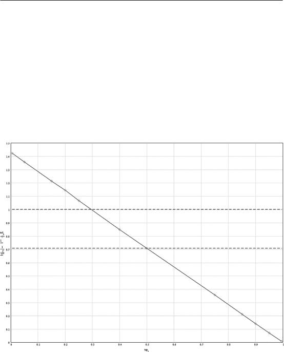
Some more Monte Carlo work, with 8000 trials per data point, revealed that there is a linear relationship between accuracy and the “tap position” of the output between R1 and R2, as shown in Figure 15.4. Plotting against division ratio would not give a straight line. With R1 = R2 the tap is at 50%, and accuracy improved by a factor of √2, as noted earlier. With a tap at about 30% (R1 = 7 kΩ,
Figure 15.4: The accuracy of the output of a resistive divider made up with components of the same tolerance varies with the divider ratio.

Passive Components for Active Crossovers 441
R2 = 3 kΩ) the accuracy is the same as the resistors used. This assessment is not applicable to potentiometers, as the two sections of the pot are not uncorrelated in value—they are highly correlated.
The two-tap divider (Figure 15.3d) and three-tap divider(Figure 15.3e) were also given a Monte Carlo work-out, though only for equal resistors. The two-tap divider has an accuracy factor of 0.404 at OUT
1 and 0.809 at OUT 2. These numbers are very close to √2/(2√3) and √2/(√3) respectively. The threetap divider has an accuracy factor of 0.289 at OUT 1, of 0.500 at OUT 2, and of 0.864 at OUT 3. The middle figure is clearly 1/2 (twice as many resistors as a one-tap divider, so √2 times more accurate), while the first and last numbers are very close to √3/6 and √3/2 respectively. It would be helpful if someone could prove analytically that the factors proposed are actually correct.
For the inverting amplifier of Figure 15.3f, the values of R1 and R2 are completely uncorrelated, and so the accuracy of the gain is always √2 worse than the tolerance of each resistor, assuming the tolerances are equal. The nominal resistor values have no effect on this. We therefore have the interesting situation that a non-inverting amplifier will always be equally or more accurate in its gain than an inverting amplifier. So far as I know this is a new result. Maybe it will be useful.
Resistor Noise: Johnson and Excess Noise
All resistors, no matter what their method of construction, generate Johnson noise. This is white noise, which has equal power in equal absolute bandwidth, i.e. with the bandwidth measured in Hz, not octaves. There is the same noise power between 100 and 200 Hz as there is between 1100 and 1200
Hz. The level of Johnson noise that a resistor generates is determined solely by its resistance value, the absolute temperature (in degrees Kelvin), and the bandwidth over which the noise is being measured. For our purposes the temperature is 25 °C and the bandwidth is 22 kHz, so the resistance is really the only variable. The level of Johnson noise is based on fundamental physics and is not subject to modification, negotiation, or any sort of rule-bending . . . however, you might want to look up “load synthesis”, in which a high-value resistor is made to act like a low-value resistor but still having the low Johnson current noise of the high-value resistor. [9] Sometimes Johnson noise from resistors places the limit on how quiet a circuit can be, though more often the noise from the active devices is dominant. It is a constant refrain in this book that resistor values should be kept as low as possible, without introducing distortion by overloading the circuitry, in order to minimise the Johnson noise contribution and the effects of opamp current noise.
The rms amplitude of Johnson noise is calculated from the classic equation:
|
vn = 4kTRB |
15.4 |
Where: |
|
|
vn is the rms noise voltage |
T is absolute temperature in °K |
B is the bandwidth in Hz |
k is Boltzmann’s constant |
R is the resistance in Ohms |
|
The thing to be careful with here is to use Boltzmann’s constant (1.380662 × 10⁻²³), and NOT the Stefan-Boltzmann constant (5.67 10−08), which relates to black-body radiation, has nothing to do with

442 Passive Components for Active Crossovers
resistors, and will give some impressively wrong answers. The voltage noise is often left in its squared form for ease of RMS-summing with other noise sources.
The noise voltage is inseparable from the resistance, so the equivalent circuit is of a voltage source in series with the resistance present. Johnson noise is usually represented as a voltage, but it can also be treated as a Johnson noise current, by means of the Thevenin-Norton transformation, [10] which gives the alternative equivalent circuit of a current source in shunt with the resistance. The equation for the noise current is simply the Johnson voltage divided by the value of the resistor it comes from:
in = vn /R. |
15.5 |
Excess resistor noise refers to the fact that some resistors, with a constant voltage drop across them, generate extra noise in addition to their inherent Johnson noise. This is a very variable quantity, but is essentially proportional to the DC voltage across the component; the specification is therefore in the form of a “noise index” such as “1 uV/V”. The uV/V parameter increases with increasing resistor value and decreases with increasing resistor size or power dissipation capacity. Excess noise has a 1/f frequency distribution. It is usually only of interest if you are using carbon or thick-film resistors— metal film and wirewound types should have little or no excess noise.Arough guide to the likely range for excess noise specs is given in Table 15.13
One of the great benefits of opamp circuitry is that it allows simple dual-rail operation, and so it is noticeably free of resistors with large DC voltages across them; the offset voltages and bias currents involved are much too low to cause measurable excess noise. If you are designing an active crossover on this basis, then you can probably forget about the issue. If, however, you are using discrete transistor circuitry, it might possibly arise; specifying metal film resistors throughout, as you no doubt would anyway, should ensure you have no problems.
To get a feel for the magnitude of excess resistor noise, consider a 100 kΩ 1/4 W carbon film resistor with a steady 10 V across it. The manufacturer’s data gives a noise parameter of about 0.7 uV/V, and so the excess noise will be of the order of 7 uV, which is −101 dBu. That could definitely be a problem in a low-noise preamplifier stage.
Table 15.13: Resistor excess noise.
Type |
Noise Index uV/V |
|
|
Metal film TH |
0 |
Carbon film TH |
0.2–3 |
Metal oxide TH |
0.1–1 |
Thin film SM |
0.05–0.4 |
Bulk metal foil TH |
0.01 |
Wirewound TH |
0 |
|
|
(Wirewound resistors are normally considered to be completely free of excess noise.)